별의 역학도 플라즈마 [2]물리학 분야와 관련이 있다.두 분야는 20세기 초 비슷한 시기에 상당한 발전을 거쳤고, 두 분야 모두 유체역학 분야에서 원래 개발된 수학적 형식주의를 차용했다.
강착 원반과 항성 표면에서는 고밀도 플라즈마 또는 가스 입자가 매우 자주 충돌하며, 충돌은 자기장 하에서 균등화 및 점도를 발생시킵니다.부착 원반과 항성 대기의 크기가 다양하며, 둘 다 엄청난 양의 미세한 입자 질량으로 이루어져 있습니다. ( {\
( - pc / km M / ){ (^ { - { \ text { } / { \ { km / } , 1 { \ }= m { } } } 。
m_ 태양과 같은 별 또는 km 크기의 항성 블랙홀 주변,
(pc / km M / p ){ ( text{{\}/ m_ 은하의 중심에 있는 태양질량 블랙홀(약 AU 크기).
시스템 교차 시간 척도는 항성 역학에서 긴데, 여기서 쉽게 알아차릴 수 있습니다.
시간이 길다는 것은 강착 원반의 가스 입자와 달리 은하 원반의 별들은 항성 수명 동안 충돌을 거의 볼 수 없다는 것을 의미합니다.그러나 은하는 은하단에서 가끔 충돌하고 별들은 가끔 성단에서 가까이서 마주칩니다.
경험에 비추어 볼 때, 관련된 일반적인 척도입니다(P.C.의 상부 참조).Budassi의 우주 로그 는(N) {입니다
( c/ k / , M / )( \ ( \ { // } , { \ / 1000 ) ) 。
( c / k / , M / 11) ( \ \ sim ( \ { kpc / / } , { } M _ { \ / ^ { 11} ) 、
총알 의 중성미자에 대한 M_nu}}}. 이는 N = 1000개의 은하로 이루어진 병합 시스템입니다
케플러 문제와 3체 문제와의 연관성
표면적인 수준에서, 모든 항성 역학은 뉴턴의 제2법칙에 의해 N-체 문제로 공식화될 수 있으며, 여기서 N개의 구성원으로 구성된 고립된 항성계의 내부 상호작용에 대한 운동 방정식(EOM)은 다음과 같이 기록될 수 있다.
여기 N-body system에서, 모든({{i})는 구성원의 중력 전위에 의해 영향을 받습니다.
실제로, 최고 성능의 컴퓨터 시뮬레이션을 제외하고, 이러한 방식으로 대규모 N 시스템의 미래를 엄격하게 계산하는 것은 가능하지 않습니다.또한 이 EOM은 직관력이 거의 없습니다.역사적으로, 항성 역학에서 사용된 방법은 고전 역학과 통계 역학 분야 모두에서 비롯되었다.본질적으로, 항성 역학의 근본적인 문제는 N-체 문제인데, 여기서 N개의 구성원은 주어진 항성계의 구성원을 말합니다.항성계에 많은 수의 물체가 존재할 경우, 항성역학에서는 여러 궤도의 전역적, 통계적 특성뿐만 아니라 개별 [1]궤도의 위치와 속도에 대한 특정 데이터도 다룰 수 있습니다.
중력 전위장의 개념
별의 역학에는 상당한 수의 별의 중력 잠재력이 포함되어 있습니다.이 별들은 궤도들이 서로 결합된 상호작용에 의해 결정되는 점 질량으로 모델링될 수 있다.일반적으로 이러한 점 질량은 은하단이나 구상성단과 같은 다양한 성단이나 은하에 있는 별들을 나타냅니다.매 초마다 시스템의 모든 점 질량 전위를 더함으로써 시스템의 중력 전위를 얻지 않고도, 항성 역학자들은 계산적으로 [3]저렴하게 유지하면서 시스템을 정확하게 모델링할 수 있는 잠재적 모델을 개발합니다.시스템의 중력 퍼텐셜(\는 다음과 같이 가속도 및 g(\displaystyle {g와 관련이 있습니다.
서 Ve ( ){ V _ { ( ) takes 、 ( \ _ { 0 )、 2 0 ( \ ) where where the where where where where 、 \ _ { } is whereescescescescescescescescescescescescescesc where where whereescescescescescescescesc esc where where where where where where where where where where where where where where where where where where where where where where where where where where where where where where where where중력은 구 내부에서는 고조파 발진기의 복원력과 같고, 밖에서는 헤비사이드 함수에 의해 설명되는 케플러의 복원력과 같다.
구면 포아송 방정식을 사용하여 해당 밀도를 계산하여 V 00})을 수정할 수 있습니다.
봉인된 덩어리가 있는 곳
따라서 잠재적 모델은 r r 총 M 의 균일한 구에 해당합니다.
주요 개념
운동 방정식과 포아송 방정식도 좌표계와 물리적 시스템의 대칭성에 따라 비구면 형태를 취할 수 있지만 본질은 동일합니다.은하계나 구상성단에 있는 별들의 움직임은 주로 멀리 있는 다른 별들의 평균 분포에 의해 결정됩니다.항성과의 만남은 이완, 질량 분리, 조력, 그리고 시스템 구성원의 [4]궤적에 영향을 미치는 동적 마찰과 같은 과정을 수반합니다.
상대론적 근사
위의 뉴턴 EOM과 포아송 방정식에는 세 가지 관련 근사치가 있습니다.
SR 및 GR
첫째, 위의 방정식은 상대론적 보정을 무시한다, 그것은 순서이다.
전형적인 별의 3차원 속도인 는 빛의 속도보다 훨씬
에딩턴 한계
둘째, 항성계에서는 일반적으로 무중력이 무시할 수 있습니다.예를 들어, 전형적인 별 근처에서 수소 원자나 이온에 대한 복사 대 중력의 비율,
따라서 질량 {\의 발광 O형 별 주변 또는 에딩턴 한계에서 가스가 발생하는 블랙홀 주변은 제외한다면 방사력은 일반적으로 무시할 수 있다. 따라서 에딩턴 한계 대 질량비 L / Mδ {\}/은 {\}에 의해 정의된다(\ Q1
손실 원뿔
셋째, 블랙홀에서 슈바르츠실트 반경 몇 개 안에 들어가면 별이 삼켜질 수 있습니다.이 손실 반경은 다음과 같습니다.
손실 원뿔은 작은 고체 각도(속도의 원뿔) 내에서 블랙홀을 겨냥한 유입 입자를 고려하여 시각화할 수 있습니다. 1{ 1}의 입자는 단위 질량당 각운동량이 작다.
각운동량이 작기 때문에( 에) 입자가 회전할 수 있는 충분한 장벽이 손실에는 없습니다.
유효 잠재력
뉴턴 중력에서는 항상 양의 무한대입니다.단, GR에서는 2(\}) 에서 마이너스 무한대로 곤두박질쳤다. J4 Mc. \ J \ {) 。
엄격한 GR 처리를 하지 않고 이 (\을 확인할 수 있습니다. 유효 전위는 변곡점 δ ( 손실 ( 손실0 {\loss}}} =\\\{loss}}\\\\\인 마지막 안정 원궤도를 계산한다.슈바르츠실트 블랙홀의 근사 고전적 전위를 이용한 loss
조석 교란 반지름
별은 소위 힐의 블랙홀 반경 안에 들어오면 무거운 블랙홀에 의해 조석적으로 찢어질 수 있습니다. 그 안에서 별의 표면 중력은 [5]블랙홀로부터의 조력에 의해 감소합니다.
인 M ( 8.5 ) M {\{\bullet } ( 파괴 반지름
여기서 0.001pc는 가장 밀도가 높은 항성계의 항성 간격이다(예: 은하 중심부의 핵성단).따라서 (주계열성) 별들은 일반적으로 은하나 성단 환경에서 가장 강한 블랙홀 조수에 의해 방해를 받기에는 내부가 너무 작고 간격이 너무 멀다.
영향권 반지름
블랙홀의 (훨씬 더 큰) 단면 s2 {\}^{2에 들어가면 상대 속도 V의 m{\ m 입자가 편향됩니다.소위 영향권이라고 하는 이 범위는 Q와 같은 퍼지 ln 스타일)에 의해 느슨하게 정의됩니다
태양과 같은 별이라면
즉, 표면 탈출 속도가 높기 때문에 별은 블랙홀과의 일반적인 조우에서 조류가 흐트러지거나 물리적으로 부딪히거나 충돌하지 않습니다.
모든 태양질량별로부터 은하단 내 은하간 내부속도와 비슷하며 일반적인 내부속도보다 크다.
모든 성단 내부와 은하에 있습니다.
별 손실 원뿔과 중력 가스 부착 물리 사이의 연관성
질량 M의 무거운 블랙홀이 (축소된 열음속 (\ 및 밀도 가스 \gas의 소산 가스 속을 이동하고 있다고 가정하면 질량 M의 모든 가스 입자는 상대 을 전달할 가능성이 높습니다. ( \ style _ { \ )반경의 단면 내에 있는 경우 BH에 대한 V ( \ displaystyle mV _ { \ bullet } )
블랙홀이 흐름 속도의 을 잃는 에서의 에 들어가는 대부분의 가스 입자를 포착하는 과정인본디 질량이 두 배로 증가하여 가스 충돌에 의해 운동에너지가 소멸되어 th에 떨어진다e 블랙홀가스 포집률은
(움직이는) 블랙홀에 의한 별 조석 교란과 별 포획으로 돌아가서 하면 가스와 별에서 BH의 증가율을 M s+ loss { { M _ \ 으로 요약할 수 있습니다.와 함께,
왜냐하면 블랙홀은 영향권을 통과하는 별/가스 입자의 일부/대부분을 소비하기 때문이다.
중력 동적 마찰
총질량)의 성단에서 Mµ {\의 무거운 블랙홀이 별들이 랜덤하게 움직이는 배경에 대해 평균 밀도를 갖는다고 가정하자.
표준 R(\ R 이내입니다.
직관은 중력이 가벼운 물체의 가속을 유발하고 운동량과 운동 에너지를 얻는다고 말한다.에너지와 운동량의 보존에 의해, 무거운 물체는 보상하는 양만큼 느려질 것이라고 결론지을 수 있다.고려 중인 물체에 운동량과 운동 에너지의 손실이 있기 때문에, 그 효과는 동적 마찰이라고 불립니다.
일정 시간 이완 후 무거운 블랙홀의 운동 에너지는 더 작은 질량의 배경 물체와 균등하게 분할되어야 합니다.블랙홀의 감속은 다음과 같이 설명할 수 있습니다.
서 t star(\는 동적 마찰 시간이라고 합니다.
동적 마찰 시간과 바이리얼라이즈된 시스템의 교차 시간 비교
음속 ({으로 이동하는 마하-1 BH를 고려합니다.따라서 Bondi s†({는 다음을 만족합니다.
여기서 음속은 G M ( -) R { { {= 4 \^{ 4 2 4 ^{ 10}=은 M M (N -) 4. R { =} \{}( \4. 주기의 절반이라는 점에 의해 고정된다.
으로 "반지름을 동적 시간 라고 합니다
가 M 0 V v V v 0 v _ { t _ { \ { fric M V { \ V { } { \ {} 을 이동한 후 한다고 가정합니다별이 BH의 Bondi 단면에 의해 영향을 받는 것은 다음과 같다.
보다 일반적으로 별의 바다의 전위(\에서 일반 Vδ {\}}에서의 BH 운동 방정식은 다음과 같이 쓸 수 있다.
서 N { N^ { \ { }}은 "직경" 교차시간당 굴절 횟수이며, 2 { { {2} \ 8} \ 、 1 1the 、 2 2 ⊙ [ ' V 4 1 1 1 1 1 \ \ \ \} \ \ [ { \ 2} \} \ } \ [ ( 1 + { V { \ bullet } \ } } \ } \ } } } { { } } } { } } { } } { } } } } } } { } } M {\} \}。일반적으로 볼 때, 무게의 1/8을 초과하지 않고 아음속를 가장자리에서 중앙으로 "전환"하는 데 시간은 약 {\dot}}} } 더 가볍고 빠른 구멍은 훨씬 더 오래 떠 있을 수 있다.
동적 마찰의 보다 엄격한 공식화
물체의 속도 변화에 대한 완전한 찬드라세카르 동적 마찰 공식은 물질장의 위상 공간 밀도에 통합되며 투명과는 거리가 멀다.
라고 쓰여 있다
어디에
는 블랙홀의 영향권 내에 있는 V d t{\ V_} 및 단면 2 {\}^의 극소 원통 부피 내의 입자 수입니다.
원거리 배경 입자의 기여에 대한 "Couloumb log" ln \ \ ln \ } 인수와 마찬가지로 여기서 ln(beaten ) ln ( \ _ { \ { } )는 HUTE보다 느린 배경 입자에 대한 기여에 대한 기여하는 요인입니다.BH에 의해 추월되는 파티클이 많을수록 BH를 끌어당기는 파티클이 많아지고 ln beated 이 커집니다.또, 시스템이 클수록 ln(\\ln \ \Lambda이 커집니다.
또한 소립자(가스 또는 다크)의 배경은 주변 매질의 질량 mnn에 따라 스케일링되는 동적 마찰을 유발할 수 있으며, 낮은 입자 질량 m은 높은 수 밀도 n으로 보상된다.질량이 큰 물체일수록 더 많은 물질이 물결로 유입될 것이다.
충돌 가스와 무충돌 별의 중력 항력을 합하면, 우리는
여기서 가스와 별에 대한 "빈" 분율은 다음과 같이 주어진다.
여기서 BH가 시간 t부터 움직이기 시작한다고 가정하고, 가스는 음속(\와 등온이며, 배경별은 맥스웰 의 을 가진다.분포 속도 spread { \ \ } velocity disp, )( \ \ \ text {) 。
흥미롭게도 (δ) ( () { G (}) mn (\ 의존성은 두 물체와 맞닿은 거대한 물체의 중력에 의해 유도되는 웨이크에 의한 중력으로부터 동적 마찰이 발생함을 시사한다.
이 힘은 또한 고단에서의 속도의 역제곱에 비례한다는 것을 알 수 있습니다. 따라서 에너지 손실의 부분 속도는 고속으로 빠르게 감소합니다.그러므로 동적 마찰은 광자와 같이 상대론적으로 움직이는 물체에 중요하지 않다.이는 오브젝트가 미디어를 통해 빠르게 이동할수록 그 뒤에 웨이크가 쌓일 시간이 줄어든다는 것을 인식함으로써 합리화할 수 있습니다.마찰은 음장벽에서 가장 높은 경향이 있으며, 서은 1 ^{ \를 합니다. _}=\{{\filen s_
항성계에 있는 별들은 강하고 약한 중력 충돌로 인해 서로의 궤도에 영향을 미칠 것이다.두 별 사이의 만남은 가장 가까운 경로에서 상호 위치 에너지가 초기 운동 에너지와 비슷하거나 미미한 경우 강하거나 약한 것으로 정의된다.강한 조우 현상은 드물며, 일반적으로 밀도가 높은 항성계에서만 중요하게 여겨집니다. 예를 들어, 지나가는 별은 구상 [7]성단의 중심핵에 있는 쌍성에 의해 방출될 수 있습니다.이것은 두 별이 떨어져 있어야 한다는 것을 의미합니다.
여기서 Virial 정리를 사용했는데, "상호 전위 에너지는 평균 두 배의 운동 에너지를 균형 잡는다" 즉, "별 쌍별 전위 에너지는 세 방향의 음속과 관련된 두 배의 운동 에너지와 균형을 맞춘다.",
서 인자 (N -) / ({N(는 쌍성간 악수 횟수이며, 평균 쌍 쌍 2 . ({\ R_}} = pi ^{약 0.41R입니다. {\ \ Q \ { } \ 화살표 \ \ \ 의 유사성도 주의해 주십시오.
자유
일반적으로(-) . R 100{ )=.19 항성계에서 강한 조우 시의 평균 자유 경로는 다음과 같다.
즉, 일반 별이 횡단면 2 스타일 에 들어오려면 약.0.의 반지름 교차가 필요합니다.따라서 강한 만남의 평균 자유시간은 R R보다 훨씬 길다.
약한 만남은 많은 구절에서 항성계의 진화에 더 심오한 영향을 미칩니다.중력 조우 효과는 릴렉스 시간의 개념으로 연구할 수 있다.이완을 보여주는 간단한 예는 다른 별과의 중력 상호작용으로 인해 별의 궤도가 바뀌는 두 개의 신체 이완입니다.
처음에 대상별은 중력장이 원래 궤도에 영향을 미치는 필드별에 가장 가까운 거리인 충격 매개변수에 수직인 속도 v의 궤도를 따라 이동합니다.뉴턴의 법칙에 따르면 대상별의 속도 변화 v\는 충격 매개 변수에서의 가속도에 가속도의 지속 시간을 곱한 값과 거의 동일합니다.
완화 시간은 § 가 v와 데 걸리는 시간 또는 작은 속도 편차가 별의 초기 속도와 같아지는 데 걸리는 시간으로 볼 수 있습니다.N개의천체(\ N로된 항성계에서 평균적인 별이 휴식을 취할 수 있는 "반지름" 교차 횟수는 대략 다음과 같습니다.
위의 평균 자유시간 추정치보다 더 엄격한 계산으로부터 강한 편향에 대한 정보를 얻을 수 있습니다.
단일 바디 시스템이나 2-바디 시스템에는 긴장을 풀 수 없기 때문에 답은 타당합니다.타임스케일 비율의 더 나은 는 N+ 1 + N 2 0. ( -)\ 입니다.123)}}}}}}}}}}}}}}}}}}}}}}}}}}}}}}}}}}}, 즉 3체, 4체, 5체, 5체, 7체, 10체, ..., ..., 42체, 72체, 140체, 210체, 210체, 210체, 550체, 3, 3, 6, 6, 6, 6, 16, …, …, …, …, …의 완화 시간은 약 16, 16, 16이다.고립된 쌍성계에는 이완이 없으며, 이완이 16개 체계의 경우 가장 빠릅니다. 궤도가 서로 흩어지기 위해서는 약 2.5개의 교차로가 필요합니다.N~ 2 - 10{\N10}-10인은 훨씬 더 부드러운 잠재성을 가지며, 일반적으로 에너지를 크게 변화시키기 위해하는 데~ lnN이 소요됩니다.
마찰과 이완의 관계
분명히 블랙홀의 동적 마찰은 완화 시간보다 약 M / M { }/만큼 훨씬 빠르지만, 이 두 가지는 블랙홀 군집의 경우 매우 유사합니다.
예를 들어 N , p - p c, / - k / { N =^ { } , ~R= \ { 1 - 10 ^ { } pc , ~ V = \ { 1 / 1 / 10 / s / 3 k m ^ { 1 . 3인 성단의 경우 100。따라서 이러한 항성 또는 은하단에서 구성원의 조우량은 일반적인 10 Gyr 수명 동안 중요합니다.
반면, 예를 들어, - {\ 10^{11}}의 별을 가진 일반적인 은하는 - k c m/ ~ M y r \ { \ \ { 1 \ mathkrm { \ 1 \ 1 . 100 그리고 그들의 휴식 시간은 우주의 나이보다 훨씬 길다.이는 수학적으로 부드러운 기능을 가진 은하의 잠재력을 모델링하는 것으로, 일반적인 은하의 일생 동안 두 개의 물체와 마주치는 것을 무시합니다.그리고 이러한 전형적인 은하 안에서 10 Gyr 허블 시간에 걸친 항성 블랙홀의 동적 마찰과 강착은 블랙홀의 속도와 질량을 아주 작은 부분만 변화시킵니다.
블랙홀이 전체 은하 의 0.1% 미만인 경우 ~ 6 - }\10^{}. {\{\bullet }\xy 퍼텐셜
동적 마찰 또는 완화 시간은 무충돌 입자 시스템과 충돌 입자 시스템을 식별합니다.일반적인 별은 초기 궤도 크기 t/ 이완1(\ t1)만큼 벗어나기 때문에 이완 시간보다 훨씬 짧은 시간 척도의 역학은 효과적으로 충돌하지 않습니다.이들은 또한 대상별이 점질량 전위의 합계가 아닌 부드러운 중력 전위와 상호작용하는 시스템으로 확인됩니다.은하에 축적된 두 개의 신체 이완 효과는 질량 분리로 알려져 있는데, 질량 분리는 성단의 중심 근처에 더 많은 무거운 별들이 모이는 반면, 질량이 적은 별들은 성단의 바깥쪽으로 밀려납니다.
충돌 및 무충돌 프로세스에서의 연속성 지표의 구면-소 요약
중력계에서 입자의 다소 복잡한 상호작용에 대한 세부사항을 살펴본 후, 적당한 가격으로 일반적인 주제를 축소하고 추출하는 것이 항상 도움이 됩니다. 따라서 더 가벼운 부하로 계속 진행하십시오.
첫 번째 중요한 개념은 '중력 균형 운동'으로, 퍼터버 근처와 배경 전체에 대한 것입니다.
by consistently omitting all factors of unity , , etc for clarity, approximating the combined mass and being ambiguous whether the geometry of the system is a thin/thick gas/stellar disk or a (non)-uniform stellar/dark sphere with or without a boundary, and about the subtle distinctions among the kinetic energies from the local Circular rotation speed, radial infall speed , globally isotropic or anisotropic random motion in one or three directions, or the (non)-uniform isotropic Sound speed to emphasize of the logic behind the order of magnitude of the friction time scale.
둘째, 시스템의 모든 일반 수량 Q에 대해구면 소 스타일의 연속성방정식으로 지금까지의 충돌 및 무충돌 가스/별 또는 암흑 물질에 대한 다양한 프로세스를 재점검하거나 매우 느슨하게 요약할 수 있습니다.
where the sign is generally negative except for the (accreting) mass M, and the Mean free path or the friction time can be due to direct molecular viscosity from a physical collision Cross section, or due to gravitational scattering (bending/focusing/Sling shot) of particles; generally the influenced area is the greatest of the competing processes of Bondi accretion, Tidal disruption, and Loss cone capture,
예: Q가 퍼터버의 Q { Q인 경우, (가스/별) 부착률을 통해 동적 마찰 시간을 추정할 수 있습니다.
where we have applied the relations motion-balancing-gravity.
한계에서 퍼트리버는 N개 배경 입자 중 (M∙ {\M_{\m에 불과하며 마찰 시간은 (중요) 릴랙세이션 시간으로 식별됩니다.다시 모든 쿨롱 로그 등은 이들 정성 방정식의 추정을 변경하지 않고 억제된다.
나머지 별의 역학에서는 중력 마찰과 백일해체의 이완을 무시하고 N µ({ N 내에서 작업함으로써 주로 작업 예제를 통해 정확한 계산에 일관되게 임할 것입니다. 비록 허블 시간 척도가 14Gyrs Hubble 시간 척도의 대부분의 은하에서 사실로 추정됩니다.s는 때때로 [7]성단의 일부 성단 또는 은하단에 대해 위반됩니다.
여기에서는 Stellar dynamics와 Accculation disc 물리학의 몇 가지 주요 방정식에 대한 간략한 1페이지 분량의 요약본을 보여 줍니다.
Stellar dynamics 주요 개념 및 방정식
통계역학 및 플라즈마 물리학과의 연결
항성 역학의 통계적 특성은 20세기 초 제임스 진스와 같은 물리학자들이 가스의 운동 이론을 항성 시스템에 적용한 것에서 비롯됩니다.중력장 내 별계의 시간 진화를 설명하는 진 방정식은 이상적인 유체에 대한 오일러의 방정식과 유사하며, 무충돌 볼츠만 방정식에서 파생되었습니다.이것은 원래 루드비히 볼츠만에 의해 열역학계의 비평형 거동을 설명하기 위해 개발되었다.통계 역학과 유사하게, 항성 역학은 확률론적 방식으로 항성계의 정보를 캡슐화하는 분포 함수를 이용한다.단일 입자 위상 공간 분포 f ( , ,) { f ,\ , 는 다음과 같은 방식으로 정의됩니다.
where represents the probability of finding a given star with position around a differential volume and velocity around a differential velocity space volume . The distribution function is normalized (sometimes) such that integrating it over all positions and velocities will equal N, the total number of bodies of the system. For collisional systems, Liouville's theorem is applied to study the microstate of a stellar system, and is also commonly used to study the different statistical ensembles of statistical mechanics.
열 분포의 경우 표기법
의 항성역학 문헌에서는 입자의 질량이 태양질량 M {\ M_에서 통일성이므로 입자의 운동량과 속도는 동일하다는 관례를 채택하는 것이 편리하다.
예를 들어, 일정한 0~ K의 에서 공기 분자의 열 속도 분포 양성자 질량의 15배)는 맥스웰 분포를 가진다
단위당 에너지 질량이
where
및 1 k 0 /~ 0.k m/ { \ _ 1} ={ 는 맥스웰 속도 분포의 폭이며, 실내의 각 방향과 모든 곳에서 동일하며, e T0(\ \m ( ≤ ≤ 2ln)이라고 가정함)] 0 \ \ \ \ sim ( m { { 1 } ^{\ } )\ \ [ { \ m \ _ { { { } \ }^{ } \ right } \ l 0 0 0 0 0 0 0 Ferm \ 3 number number number number number number number number number number number number number number number number number number number number number number number number number number number number number number number number number number number number number number number number number레벨, 여기서
The CBE
In plasma physics, the collisionless Boltzmann equation is referred to as the Vlasov equation, which is used to study the time evolution of a plasma's distribution function.
The Boltzmann equation is often written more generally with the Liouville operator as
where is the gravitational force and is the Maxwell (equipartition) distribution (to fit the same density, same mean and rms velocity as ). The equation means the non-Gaussianity will decay on a (relaxation) time scale of , and the system will ultimately relaxes to a Maxwell (equipartition) distribution.
Whereas Jeans applied the collisionless Boltzmann equation, along with Poisson's equation, to a system of stars interacting via the long range force of gravity, Anatoly Vlasov applied Boltzmann's equation with Maxwell's equations to a system of particles interacting via the Coulomb Force.[8] Both approaches separate themselves from the kinetic theory of gases by introducing long-range forces to study the long term evolution of a many particle system. In addition to the Vlasov equation, the concept of Landau damping in plasmas was applied to gravitational systems by Donald Lynden-Bell to describe the effects of damping in spherical stellar systems.[9]
A nice property of f(t,x,v) is that many other dynamical quantities can be formed by its moments, e.g., the total mass, local density, pressure, and mean velocity. Applying the collisionless Boltzmann equation, these moments are then related by various forms of continuity equations, of which most notable are the Jeans equations and Virial theorem.
Probability-weighted moments and hydrostatic equilibrium
Jeans computed the weighted velocity of the Boltzmann Equation after integrating over velocity space
and obtain the Momentum (Jeans) Eqs. of a opulation (e.g., gas, stars, dark matter):
The general version of Jeans equation, involving (3 x 3) velocity moments is cumbersome. It only becomes useful or solvable if we could drop some of these moments, epecially drop the off-diagonal cross terms for systems of high symmetry, and also drop net rotation or net inflow speed everywhere.
The isotropic version is also called Hydrostatic equilibrium equation where balancing pressure gradient with gravity; the isotropic version works for axisymmetric disks as well, after replacing the derivative dr with vertical coordinate dz. It means that we could measure the gravity (of dark matter) by observing the gradients of the velocity dispersion and the number density of stars.
Applications and examples
Stellar dynamics is primarily used to study the mass distributions within stellar systems and galaxies. Early examples of applying stellar dynamics to clusters include Albert Einstein's 1921 paper applying the virial theorem to spherical star clusters and Fritz Zwicky's 1933 paper applying the virial theorem specifically to the Coma Cluster, which was one of the original harbingers of the idea of dark matter in the universe.[10][11] The Jeans equations have been used to understand different observational data of stellar motions in the Milky Way galaxy. For example, Jan Oort utilized the Jeans equations to determine the average matter density in the vicinity of the solar neighborhood, whereas the concept of asymmetric drift came from studying the Jeans equations in cylindrical coordinates.[12]
Stellar dynamics also provides insight into the structure of galaxy formation and evolution. Dynamical models and observations are used to study the triaxial structure of elliptical galaxies and suggest that prominent spiral galaxies are created from galaxy mergers.[1] Stellar dynamical models are also used to study the evolution of active galactic nuclei and their black holes, as well as to estimate the mass distribution of dark matter in galaxies.
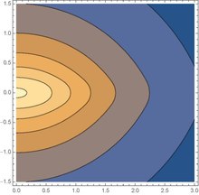
Note the somewhat pointed end of the equal potential in the (R,z) meridional plane of this R0=5z0=1 model
A unified thick disk potential
Consider an oblate potential in cylindrical coordinates
where are (positive) vertical and radial length scales. Despite its complexity, we can easily see some limiting properties of the model.
First we can see the total mass of the system is because
when we take the large radii limit , so that
We can also show that some special cases of this unified potential become the potential of the Kuzmin razor-thin disk, that of the Point mass , and that of a uniform-Needle mass distribution:
A worked example of gravity vector field in a thick disk
First consider the vertical gravity at the boundary,
Note that both the potential and the vertical gravity are continuous across the boundaries, hence no razor disk at the boundaries. Thanks to the fact that at the boundary, is continuous. Apply Gauss's theorem by integrating the vertical force over the entire disk upper and lower boundaries, we have
confirming that takes the meaning of the total disk mass.
The vertical gravity drops with
at large radii, which is enhanced over the vertical gravity of a point mass due to the self-gravity of the thick disk.
Density of a thick disk from Poisson Equation
Insert in the cylindrical Poisson eq.
which drops with radius, and is zero beyond and uniform along the z-direction within the boundary.
Note the vertically uniform thick disk density contour in this R0=5z0=1 model
Surface density and mass of a thick disk
Integrating over the entire thick disc of uniform thickness , we find the surface density and the total mass as
This confirms that the absence of extra razor thin discs at the boundaries. In the limit, , this thick disc potential reduces to that of a razor-thin Kuzmin disk, for which we can verify .
Oscillation frequencies in a thick disk
To find the vertical and radial oscillation frequencies, we do a Taylor expansion of potential around the midplane.
and we find the circular speed and the vertical and radial epicycle frequencies to be given by
Interestingly the rotation curve is solid-body-like near the centre , and is Keplerian far away.
At large radii three frequencies satisfy . E.g., in the case that and , the oscillations forms a resonance.
In the case that , the density is zero everywhere except uniform needle between along the z-axis.
If we further require , then we recover a well-known property for closed ellipse orbits in point mass potential,
A worked example for neutrinos in galaxies
For example, the phase space distribution function of non-relativistic neutrinos of mass m anywhere will not exceed the maximum value set by
where the Fermi-Dirac statistics says there are at most 6 flavours of neutrinos within a volume and a velocity volume
.
Let's approximate the distribution is at maximum, i.e.,
where such that , respectively, is the potential energy of at the centre or the edge of the gravitational bound system. The corresponding neutrino mass density, assume spherical, would be
which reduces to
Take the simple case , and estimate the density at the centre with an escape speed , we have
Clearly eV-scale neutrinos with is too light to make up the 100–10000 over-density in galaxies with escape velocity , while neutrinos in clusters with could make up times cosmic background density.
By the way the freeze-out cosmic neutrinos in your room have a non-thermal random momentum , and do not follow a Maxwell distribution, and are not in thermal equilibrium with the air molecules because of the extremely low cross-section of neutrino-baryon interactions.
A Recap on Harmonic Motions in Uniform Sphere Potential
Consider building a steady state model of the fore-mentioned uniform sphere of density and potential
where is the speed to escape to the edge .
First a recap on motion "inside" the uniform sphere potential. Inside this constant density core region, individual stars go on resonant harmonic oscillations of angular frequency with
Loosely speaking our goal is to put stars on a weighted distribution of orbits with various energies , i.e., the phase space density or distribution function, such that their overall stellar number density reproduces the constant core, hence their collective "steady-state" potential. Once this is reached, we call the system is a self-consistent equilibrium.
Example on Jeans theorem and CBE on Uniform Sphere Potential
Generally for a time-independent system, Jeans theorem predicts that is an implicit function of the position and velocity through a functional dependence on "constants of motion".
For the uniform sphere, a solution for the Boltzmann Equation, written in spherical coordinates and its velocity components is
where is a normalisation constant, which has the dimension of (mass) density. And we define a (positive enthalpy-like dimension ) Quantity
Clearly anti-clockwise rotating stars with are excluded.
It is easy to see in spherical coordinates that
Insert the potential and these definitions of the orbital energy E and angular momentum J and its z-component Jz along every stellar orbit, we have
which implies , and between zero and .
To verify the above being constants of motion in our spherical potential, we note
for any "steady state" potential.
which reduces to around the z-axis of any axisymmetric potential, where .
Likewise the x and y components of the angular momentum are also conserved for a spherical potential. Hence .
So for any time-independent spherical potential (including our uniform sphere model), the orbital energy E and angular momentum J and its z-component Jz along every stellar orbit satisfy
Hence using the chain rule, we have
i.e., , so that CBE is satisfied, i.e., our
is a solution to the Collisionless Boltzmann Equation for our static spherical potential.
A worked example on moments of distribution functions in a uniform spherical cluster
We can find out various moments of the above distribution function, reformatted as with the help of three Heaviside functions,
once we input the expression for the earlier potential inside , or even better the speed to "escape from r to the edge" of a uniform sphere Clearly the factor in the DF (distribution function) is well-defined only if , which implies a narrow range on radius and excludes high velocity particles, e.g., , from the distribution function (DF, i.e., phase space density).
In fact, the positivity carves the () left-half of an ellipsoid in the velocity space ("velocity ellipsoid"),
where is rescaled by the function or respectively.
The velocity ellipsoid (in this case) has rotational symmetry around the r axis or axis. It is more squashed (in this case) away from the radial direction, hence more tangentially anisotropic because everywhere , except at the origin, where the ellipsoid looks isotropic. Now we compute the moments of the phase space.
E.g., the resulting density (moment) is
is indeed a spherical (angle-independent) and uniform (radius-independent) density inside the edge, where the normalisation constant .
The streaming velocity is computed as the weighted mean of the velocity vector
where the global average (indicated by the overline bar) of flow implies uniform pattern of flat azimuthal rotation, but zero net streaming everywhere in the meridional plane.
Incidentally, the angular momentum global average of this flat-rotation sphere is
Note global average of centre of mass does not change, so due to global momentum conservation in each rectangular direction , and this does not contradict the global non-zero rotation.
Likewise thanks to the symmetry of , we have , , everywhere}.
Likewise the rms velocity in the rotation direction is computed by a weighted mean as follows, E.g.,
Here
Likewise
So the pressure tensor or dispersion tensor is
with zero off-diagonal terms because of the symmetric velocity distribution. Note while there is no Dark Matter in producing the previous flat rotation curve, the price is shown by the reduction factor in the random velocity spread in the azimuthal direction. Among the diagonal dispersion tensor moments, is the biggest among the three at all radii, and only near the edge between .
The larger tangential kinetic energy than that of radial motion seen in the diagonal dispersions is often phrased by an anisotropy parameter
a positive anisotropy would have meant that radial motion dominated, and a negative anisotropy means that tangential motion dominates (as in this uniform sphere).
A worked example of Virial Theorem
Twice kinetic energy per unit mass of the above uniform sphere is
which balances the potential energy per unit mass of the uniform sphere, inside which .
The average Virial per unit mass can be computed from averaging its local value , which yields
as required by the Virial Theorem. For this self-gravitating sphere, we can also verify that the virial per unit mass equals the averages of half of the potential
Hence we have verified the validity of Virial Theorem for a uniform sphere under self-gravity, i.e., the gravity due to the mass density of the stars is also the gravity that stars move in self-consistently; no additional dark matter halo contributes to its potential, for example.
A worked example of Jeans Equation in a uniform sphere
Jeans Equation is a relation on how the pressure gradient of a system should be balancing the potential gradient for an equilibrium galaxy. In our uniform sphere, the potential gradient or gravity is
The radial pressure gradient
The reason for the discrepancy is partly due to centrifugal force
and partly due to anisotropic pressure
so at the very centre, but the two balance at radius , and then reverse to at the very edge.
Now we can verify that
Here the 1st line above is essentially the Jeans equation in the r-direction, which reduces to the 2nd line, the Jeans equation in an anisotropic (aka ) rotational (aka ) axisymmetric ( ) sphere (aka ) after much coordinate manipulations of the dispersion tensor; similar equation of motion can be obtained for the two tangential direction, e.g., , which are useful in modelling ocean currents on the rotating earth surface or angular momentum transfer in accretion disks, where the frictional term is important. The fact that the l.h.s. means that the force is balanced on the r.h.s. for this uniform (aka ) spherical model of a galaxy (cluster) to stay in a steady state (aka time-independent equilibrium everywhere) statically (aka with zero flow everywhere). Note systems like accretion disk can have a steady net radial inflow everywhere at all time.
A worked example of Jeans equation in a thick disk
Consider again the thick disk potential in the above example. If the density is that of a gas fluid, then the pressure would be zero at the boundary . To find the peak of the pressure, we note that
So the fluid temperature per unit mass, i.e., the 1-dimensional velocity dispersion squared would be
Along the rotational z-axis,
which is clearly the highest at the centre and zero at the boundaries . Both the pressure and the dispersion peak at the midplane . In fact the hottest and densest point is the centre, where
A recap on worked examples on Jeans Eq., Virial and Phase space density
Having looking at the a few applications of Poisson Eq. and Phase space density and especially the Jeans equation, we can extract a general theme, again using the Spherical cow approach.
Jeans equation links gravity with pressure gradient, it is a generalisation of the Eq. of Motion for single particles. While Jeans equation can be solved in disk systems, the most user-friendly version of the Jeans eq. is the spherical anisotropic version for a static frictionless system , hence the local velocity spead everywhere for each of the three directions . One can project the phase space into these moments, which is easily if in a highly spherical system, which admits conservations of energy and angular momentum J. The boundary of the system sets the integration range of the velocity bound in the system.
In summary, in the spherical Jeans eq.,
which matches the expectation from the Virial theorem , or in other words, the kinetic energy of an equilibrium equals the average kinetic energy on circular orbits with purely transverse motion.


![{\displaystyle {\begin{aligned}\Phi (r)&\equiv \left(-V_{0}^{2}\right)+\left[{r^{2}-r_{0}^{2} \over 2r_{0}^{2}},~~1-{r_{0} \over r}\right]_{\max }\!\!\!\!V_{0}^{2}\equiv \Phi (r_{0})-{V_{e}^{2}(r) \over 2},~~\Phi (r_{0})=-V_{0}^{2},\\\mathbf {g} &=-\mathbf {\nabla } \Phi (r)=-\Omega ^{2}rH(r_{0}-r)-{GM_{0} \over r^{2}}H(r-r_{0}),~~\Omega ={V_{0} \over r_{0}},~~M_{0}={V_{0}^{2}r_{0} \over G},\end{aligned}}}](https://wikimedia.org/api/rest_v1/media/math/render/svg/9eed0a82ca69c70fbb8677ac464d6afa16ed35ca)


 균일한 구에 해당합니다.


 없습니다.
없습니다. 


![{\displaystyle \Phi (r)=-{(4GM_{\bullet }/c)^{2} \over 2r^{2}}\left[1+{3(6GM_{\bullet }/c^{2})^{2} \over 8r^{2}}\right]-{\frac {GM_{\bullet }}{r}}\left[1-{(6GM_{\bullet }/c^{2})^{2} \over r^{2}}\right].}](https://wikimedia.org/api/rest_v1/media/math/render/svg/60bb369fc622db8b3c2f7da661a35763de485737)
![{\displaystyle (1-1.5)\geq Q^{\text{tide}}\equiv {GM_{\odot }/R_{\odot }^{2} \over [GM_{\bullet }/s_{\text{Hill}}^{2}-GM_{\bullet }/(s_{\text{Hill}}+R_{\odot })^{2}]},~~~s_{\text{Hill}}\rightarrow R_{\odot }\left({(2-3)GM_{\bullet } \over GM_{\odot }}\right)^{1 \over 3},}](https://wikimedia.org/api/rest_v1/media/math/render/svg/4910f26be59eb408fb9b61e92b08abfb73374645)

![{\displaystyle \max[s_{\text{Hill}},s_{\text{Loss}}]=400R_{\odot }\max \left[\left({M_{\bullet } \over 3\times 10^{7}M_{\odot }}\right)^{1/3},{M_{\bullet } \over 3\times 10^{7}M_{\odot }}\right]=(1-4000)R_{\odot }\ll 0.001\mathrm {pc} ,}](https://wikimedia.org/api/rest_v1/media/math/render/svg/659baf1583539af79f2d2194a54f78f6f463a9fa)
 들어가면 상대 속도 V의


![{\displaystyle s_{\bullet }={G(M_{\bullet }+M_{\odot }){\sqrt {\ln \Lambda }} \over V^{2}/2}\approx {M_{\bullet } \over M_{\odot }}{V_{\odot }^{2} \over V^{2}}R_{\odot }>[s_{\text{Hill}},s_{\text{Loss}}]_{max}=(1-4000)R_{\odot },}](https://wikimedia.org/api/rest_v1/media/math/render/svg/dad9c2b8ed87ccd8391dff7c60a8d18ba0cc9ff8)


 소산 가스 속을 이동하고 있다고 가정하면 질량 M의 모든 가스 입자는 상대


![{\displaystyle {M_{\bullet } \over t_{\text{Bondi}}^{gas}}={\sqrt {{\text{ς'}}^{2}+V_{\bullet }^{2}}}(\pi s_{\bullet }^{2})\rho _{\text{gas}}=4\pi \rho _{\text{gas}}\left[{(GM_{\bullet })^{2} \over ({\text{ς'}}^{2}+V_{\bullet }^{2})^{3 \over 2}}\right]\ln \Lambda ,~~{\text{ς'}}\equiv {\text{ς}}{\sqrt {1+\gamma ^{3} \over 2(9/8)^{2/3}}},}](https://wikimedia.org/api/rest_v1/media/math/render/svg/789965d843198f310b22b3db444bf75e3cd55622)
 속도 분산의 제곱 단위의 음속이며, 스케일 조정된 음속
![{\displaystyle {\text{ς'}}^{2}\approx [{25 \over 26}+{15 \over 16}(\gamma -1)]^{2}{\text{ς}}^{2}\approx [{\text{ς}}^{2},\sigma ^{2}]_{\text{max}}}](https://wikimedia.org/api/rest_v1/media/math/render/svg/06255871b1fca706b0604287c313cb07dcc184d6)


 함께,
함께,![{\displaystyle {\dot {M}}_{\bullet }={\sqrt {{\text{ς'}}^{2}+V_{\bullet }^{2}}}(\pi s_{\bullet }^{2})\left[\rho _{\text{gas}}+{(\pi s_{\text{Hill}}^{2}+\pi s_{\text{Loss}}^{2}) \over (\pi s_{\bullet }^{2})}(n_{\text{*}}M_{\odot })\right],~~s_{\bullet }\approx {(GM_{\bullet }+Gm) \over (V_{\bullet }^{2}+{\text{ς'}}^{2})/2},}](https://wikimedia.org/api/rest_v1/media/math/render/svg/b799a93afcefc1cfa11d84fa3a8d7726a62a7bdd)


 동적 마찰 시간이라고 합니다.


 "반지름
"반지름
 이동한 후
이동한 후 


![{\displaystyle ~~n(\mathbf {x} )dx^{3}=dtV_{\bullet }(\pi s_{\bullet }^{2})n(\mathbf {x} )=dtn(\mathbf {x} )|V_{\bullet }|\pi \left[{G(m+M_{\bullet }) \over |V_{\bullet }|^{2}/2}\right]^{2}}](https://wikimedia.org/api/rest_v1/media/math/render/svg/d9d853f68fcb3d1f4c17d6af3f574a543e69b851)


![{\displaystyle {d(M_{\bullet }\mathbf {V} _{\bullet }) \over M_{\bullet }dt}=-4\pi \left[{GM_{\bullet } \over |V_{\bullet }|}\right]^{2}\mathbf {\hat {V}} _{\bullet }(\rho _{\text{gas}}\ln \Lambda _{\text{beaten}}^{gas}+mn_{\text{*}}\ln \Lambda _{\text{beaten}}^{*}).~~}](https://wikimedia.org/api/rest_v1/media/math/render/svg/4a2123e492eed2b0401fee73aba1a14e6f8fba40)
![{\displaystyle {\begin{aligned}\ln \Lambda _{\text{beaten}}^{gas}(u)&=\ln ~{\left[{1+u \over \lambda }\right]^{1 \over 2}\left[{|1-u| \over \lambda }\right]^{H[u-\lambda -1]-H[1-\lambda -u] \over 2} \over \exp {[u+\lambda ,1]_{\min }^{2}-[u-\lambda ,1]_{\min }^{2} \over 4\lambda }},\\&\approx \ln \left[{{\sqrt {(u^{3}-1)^{2}+\lambda ^{3}}}+u^{3}-1 \over {\sqrt {1+\lambda ^{3}}}-1}\right]^{1 \over 3},~~u\equiv {|V_{\bullet }|t \over {\text{ς'}}t},~~\lambda \equiv ({s_{\bullet } \over {\text{ς'}}t})\\{\ln \Lambda _{\text{beaten}}^{*} \over \ln \Lambda }&\equiv \int _{0}^{|mV_{\bullet }|}\!\!\!\!{(4\pi p^{2}dp)e^{-{p^{2} \over 2(m\sigma )^{2}}} \over ({\sqrt {2\pi }}m\sigma )^{3}}\left.\right|_{p=m|v|}\approx {|\mathbf {V} _{\bullet }|^{3} \over |\mathbf {V} _{\bullet }|^{3}+3.45\sigma ^{3}},\\\ln \Lambda &=\int {d\mathbf {x_{1}} ^{3}~n(\mathbf {x_{1}} ) \over |\mathbf {x_{1}} -\mathbf {x} |(s_{\bullet }^{2}+|\mathbf {x_{1}} -\mathbf {x} |^{2})n(\mathbf {x} )}\approx \ln {\sqrt {1+\left({0.123NM_{\odot } \over M_{\bullet }}\right)^{2}}},\end{aligned}}}](https://wikimedia.org/api/rest_v1/media/math/render/svg/247d088606e1bcbd80b7f9b66ed420f0f49950c3)


 쌍성간 악수 횟수이며, 평균 쌍


 반지름 교차가 필요합니다.따라서 강한 만남의 평균 자유시간은


![{\displaystyle s^{2}\approx \max \left[{\text{Bondi radius}}~s_{\bullet },{\text{Tidal radius}}~s_{\text{Hill}},{\text{physical size}}~s_{\text{Loss cone}}\right]^{2}.}](https://wikimedia.org/api/rest_v1/media/math/render/svg/95316105e859cb6c60d5526938de3a7192868f20)


 맥스웰 속도 분포의 폭이며, 실내의 각 방향과 모든 곳에서 동일하며,
![{\textstyle \mu \sim (m\sigma _{1}^{2})\ln \left[n_{0}\left({{\sqrt {2\pi }}\hbar \over m\sigma _{1}}\right)^{3}\right]\ll 0}](https://wikimedia.org/api/rest_v1/media/math/render/svg/f4ea8a05a3994698d3116a5b7e7cfb34574bf28c)


![{\displaystyle {1 \over \rho _{p}}\int \!\left\{\mathbf {v} _{p}{d[f_{p}m_{p}] \over dt}-\langle {\mathbf {v} }\rangle _{p}{d[f_{p}m_{p}] \over dt}\right\}d^{3}\mathbf {v} =0,}](https://wikimedia.org/api/rest_v1/media/math/render/svg/a53c2679d041b02627de3a35bb1fb0a06a895161)

![{\displaystyle {\begin{aligned}\overbrace {\left({\partial \over \partial t}+\sum _{j=1}^{3}\langle {v_{j}^{p}}\rangle {\partial \over \partial x_{j}}\right)\langle {v_{i}^{p}}\rangle } ^{{\dot {\langle {v}\rangle }}_{i}^{p}}&\underbrace {=} _{EoM}\overbrace {-\partial \Phi (t,\mathbf {x} ) \over \partial x_{i}} ^{g_{i}\sim O(-GM/R^{2})}~~\underbrace {-} _{\text{balance}}^{\text{pressure}}~~\sum _{j=1}^{3}{\partial \over \rho ^{p}\partial x_{j}}\overbrace {[\underbrace {\rho ^{p}(t,\mathbf {x} )} _{\int _{\infty }\!\!\!\!m_{p}f_{p}d^{3}\mathbf {v} }\underbrace {\sigma _{ji}^{p}(t,\mathbf {x} )} _{O(c_{s}^{2})}]} ^{\int \limits _{\infty }\!\!d\mathbf {v} ^{3}(\mathbf {v} _{j}-\langle {v}\rangle _{j}^{p})(\mathbf {v} _{i}-\langle {v}\rangle _{i}^{p})m_{p}f_{p}}-{\underbrace {\langle {v_{i}^{p}}\rangle \overbrace {[{\dot {m}}_{p}/m_{p}]} ^{1/t|_{{\text{visc}}~m_{p}=M_{\text{gas}}}^{\text{fric}}}} _{\text{snow.plough}}},\\0&=-{\partial \Phi (t,\mathbf {x} ) \over \partial x_{i}}-{\partial (n\sigma ^{2}) \over n\partial x_{i}},~~{\text{hydrostatic isotropic velocity, no flow and friction }}.\end{aligned}}}](https://wikimedia.org/api/rest_v1/media/math/render/svg/c61a4c41bc525461582c143e4befece23a8abb76)
![{\displaystyle {\begin{aligned}\Phi (R,z)&={GM_{0} \over 2z_{0}}\left[2\sinh ^{-1}\!\!Q-\sinh ^{-1}\!\!Q_{+}-\sinh ^{-1}\!\!Q_{-}\right]\\&={GM_{0} \over 2z_{0}}\log {({\sqrt {1+Q^{2}}}+Q)^{2} \over \left[{\sqrt {1+Q_{+}^{2}}}+Q_{+}\right]\left[{\sqrt {1+Q_{-}^{2}}}+Q_{-}\right]},\\Q_{\pm }&\equiv {R_{0}+\left|~|z|\pm z_{0}~\right| \over R},\\Q&\equiv {R_{0}+[0,|z|-z_{0}]_{\max } \over R},\\\end{aligned}}}](https://wikimedia.org/api/rest_v1/media/math/render/svg/0f6b5ec77f105dda2b9591a11d9a2ed7d92d6484)


![{\displaystyle \Phi _{UN}^{R_{0}=0}(R,z)={GM_{0} \over 2z_{0}}\left[2\sinh ^{-1}\!\!{(0,|z|-z_{0})_{\max } \over R}-\sinh ^{-1}\!\!{z_{0}+|z| \over R}-\sinh ^{-1}\!\!{\left|~z_{0}-|z|~\right| \over R}\right].}](https://wikimedia.org/api/rest_v1/media/math/render/svg/3743c212edf4ddd493f52da9acab8d23d4e154e4)
![{\displaystyle g_{z}(R,z)=-\partial _{z}\Phi (R,z)=-{GM_{0}z \over 2z_{0}^{2}}\left[{1 \over {\sqrt {R_{0}^{2}+R^{2}}}}-{1 \over {\sqrt {(R_{0}+2z_{0})^{2}+R^{2}}}}\right],~~z=\pm z_{0},}](https://wikimedia.org/api/rest_v1/media/math/render/svg/85e8e5dfd14cd9e91e73660a071b6c2ff7b8e0c1)


![{\displaystyle (R\omega )^{2}\equiv V_{\text{cir}}^{2}=\left[{(1+R_{0}/z_{0})GM_{0} \over {\sqrt {R^{2}+(R_{0}+z_{0})^{2}}}}-{(R_{0}/z_{0})GM_{0} \over {\sqrt {R^{2}+R_{0}^{2}}}}\right],}](https://wikimedia.org/api/rest_v1/media/math/render/svg/ab0a0d0d25dfa481b2c6e5a0f9a69ed997fb2f82)


![{\textstyle \left.\left[\omega ,\nu ,\kappa ,{\sqrt {4\pi G\rho }}\right]\right|_{R\to \infty }\to [1,1+R_{0}/z_{0},1,R_{0}/z_{0}]^{1 \over 2}{\sqrt {GM_{0} \over R^{3}}}}](https://wikimedia.org/api/rest_v1/media/math/render/svg/42a531ed2991a5baa9cee1b926a00ad9654fe270)


![{\displaystyle dv^{3}=(dp/m)^{3}=[(2\pi \hbar /dx)/m]^{3},}](https://wikimedia.org/api/rest_v1/media/math/render/svg/d8c739464e042aa32afa31d5f1a61547b12870ac)


![{\displaystyle \rho (r)\leq \rho (0)\rightarrow {m^{4}V_{0}^{3} \over \pi ^{2}\hbar ^{3}}\approx m_{\mathrm {eV} }^{4}V_{200}^{3}\times {\text{[Cosmic Critical Density]}}.}](https://wikimedia.org/api/rest_v1/media/math/render/svg/97a92535b1a4d440b298facc0dbc170662b609a7)


![{\displaystyle Q[\mathbf {x} ,\mathbf {v} ]\equiv \left[0,\left(-V_{0}^{2}-E\right)+{J^{2} \over 2r_{0}^{2}}\right]_{\max }\left[{J_{z} \over |J_{z}|},0\right]_{\max }.}](https://wikimedia.org/api/rest_v1/media/math/render/svg/4eaa0b5c7bb5700290069ac4235f5a7e903e55aa)


![{\displaystyle 2Q={\text{Heaviside}}\left({V_{\varphi } \over |V_{\varphi }|}\right)\times \left[V_{0}^{2}\left(1-{r^{2} \over r_{0}^{2}}\right)-V_{r}^{2}-\left(1-{r^{2} \over r_{0}^{2}}\right){\left(V_{\theta }^{2}+V_{\varphi }^{2}\right)},0\right]_{\max },}](https://wikimedia.org/api/rest_v1/media/math/render/svg/e24d2b8e9e6709fcd0414792e9666ae1c75d6350)


![{\displaystyle dJ_{z}/dt=0+[(V_{y})V_{x}+(-V_{x})V_{y}]-\left[(-y){x \over R}{\partial \Phi (R,z) \over \partial R}+(x){y \over R}{\partial \Phi (R,z) \over \partial R}\right]=0}](https://wikimedia.org/api/rest_v1/media/math/render/svg/7b6e0053da5b676a3ef1787106b937541b698598)


![{\displaystyle dE[\mathbf {x} ,\mathbf {v} ]/dt=dJ[\mathbf {x} ,\mathbf {v} ]/dt=dJ_{z}[\mathbf {x} ,\mathbf {v} ]/dt=0.}](https://wikimedia.org/api/rest_v1/media/math/render/svg/d6ecaf5291ffe822ad6b0ce675e5977367730b52)
![{\displaystyle {d \over dt}Q(E[\mathbf {x} ,\mathbf {v} ],J[\mathbf {x} ,\mathbf {v} ],J_{z}[\mathbf {x} ,\mathbf {v} ])={\partial Q \over \partial E}{dE \over dt}+{\partial Q \over \partial J_{z}}{dJ_{z} \over dt}+{\partial Q \over \partial J}{dJ \over dt}=0,}](https://wikimedia.org/api/rest_v1/media/math/render/svg/b64fb6518d6bcf1dbc8459392f2fce7c0b28a054)
![{\textstyle {d \over dt}f=f'(Q){dQ[\mathbf {x} ,\mathbf {v} ] \over dt}=0}](https://wikimedia.org/api/rest_v1/media/math/render/svg/e72d03f6aa902d08db4142ed73f4e89a87e599c1)
![{\displaystyle f(\mathbf {x} ,\mathbf {v} )=f(E[\mathbf {x} ,\mathbf {v} ],J[\mathbf {x} ,\mathbf {v} ],J_{z}[\mathbf {x} ,\mathbf {v} ])}](https://wikimedia.org/api/rest_v1/media/math/render/svg/05fe4d686a4b68db9cb8b76122669658217c5e4b)


![{\displaystyle {V_{e}(|\mathbf {r} |) \over {\sqrt {2Q}}}={\sqrt {\max[0,{1 \over 1-q}]}}}](https://wikimedia.org/api/rest_v1/media/math/render/svg/84cdc0dcb010a42d5e43d11f8bda2ef6bd1dfdb2)


![{\displaystyle [V_{r},V_{\theta },V_{\varphi }]}](https://wikimedia.org/api/rest_v1/media/math/render/svg/433a2094098154be05aee6da6d49cdaf61babde1)


![{\displaystyle {\begin{aligned}\langle \mathbf {V} \rangle (\mathbf {x} )&\equiv {\int fd\mathbf {V} ^{3}\mathbf {V} \over \int fd\mathbf {V} ^{3}}\\&={1 \over \rho }\int fd\mathbf {V} ^{3}[V_{r},V_{\theta },V_{\varphi }]{C_{0}V_{0}^{2}(2Q)^{-1/2}}\\&=\left[{\int _{-1}^{1}\!\!u_{r}...du_{r},~~\int _{-1}^{1}\!\!u_{\theta }...du_{\theta },~~\int _{0}^{1}(2du_{r})\int _{0}^{\sqrt {1-u_{r}^{2}}}\!\!(2du_{\theta })\int _{0}^{\sqrt {1-u_{r}^{2}-u_{\theta }^{2}}}\!\!\!\!\!\!\!\!\!\!{du_{\varphi }u_{\varphi }V_{0} \over (1-u_{r}^{2}-u_{\theta }^{2}-u_{\varphi }^{2})^{1/2}} \over \int _{0}^{1}(2\pi UdU)\int _{0}^{\sqrt {1-U^{2}}}du_{\varphi }(1-U^{2}-u_{\varphi }^{2})^{-1/2}}\right]\\&=\left[0,0,{4V_{0} \over 3\pi }\right]={\overline {\mathbf {V} (\mathbf {x} )}},\end{aligned}}}](https://wikimedia.org/api/rest_v1/media/math/render/svg/5fcd385f83559d4aae2a2b6f9b3b21e9b212e875)

![{\displaystyle {\overline {\mathbf {r} \times \langle \mathbf {V} \rangle }}=\int _{0}^{r_{0}}{(\rho 4\pi r^{2}dr) \over M_{0}}[0,0,r\langle V_{\varphi }\rangle ]=[0,0,{3r_{0} \over 4}{\overline {V_{\varphi }}}].}](https://wikimedia.org/api/rest_v1/media/math/render/svg/836d4da6c14a9ba0881e82d78d989cb33deb9235)


![{\displaystyle {\begin{aligned}\sigma _{ij}^{2}(\mathbf {r} )=&{P_{ij}(\mathbf {r} ) \over \rho (\mathbf {r} )}\\=&\langle \mathbf {V} _{i}\mathbf {V} _{j}\rangle -\langle \mathbf {V} _{i}\rangle \langle \mathbf {V} _{j}\rangle \\=&{\begin{bmatrix}\left[1-({r \over r_{0}})^{2}\right]\left({V_{0} \over 2}\right)^{2}&0&0\\0&\left({V_{0} \over 2}\right)^{2}&0\\0&0&\left[1-({8 \over 3\pi })^{2}\right]\left({V_{0} \over 2}\right)^{2}\end{bmatrix}}\end{aligned}}}](https://wikimedia.org/api/rest_v1/media/math/render/svg/280c5016c4c9601b6621346eeb8d32dfe2e48cb2)


![{\displaystyle {\begin{aligned}{\partial \langle V_{r}\rangle \over \partial t}&=(-\sum _{i=x,y,z}V_{i}\partial _{i}\langle V_{r}\rangle )-{\cancel {\langle V_{r}\rangle \over t_{\text{fric}}}}-\nabla _{r}\Phi +\sum _{i=x,y,z}{-\partial _{i}(n\sigma _{ir}^{2}) \over n}\\&={{\bar {V}}_{\theta }^{2}+{\bar {V}}_{\varphi }^{2}-2{\bar {V}}_{r}^{2} \over r}-0-{\partial \Phi \over \partial r}+\left[-{d(\rho \sigma _{r}^{2}) \over \rho dr}+{\sigma _{\theta }^{2}+\sigma _{\varphi }^{2}-2\sigma _{r}^{2} \over r}\right]\\&={0+(0.4244V_{0})^{2}-2\times 0 \over r}-(\Omega ^{2}r)+\\&\left[{\Omega ^{2}r \over 2}+{(0.5V_{0})^{2}+(0.2643V_{0})^{2}-2\times 0.25\Omega ^{2}(r_{0}^{2}-r^{2}) \over r}\right]\\&=0.\end{aligned}}}](https://wikimedia.org/api/rest_v1/media/math/render/svg/6e1ffc39f7450b92e5d0f5726c2e49b32499bdd6)


![{\displaystyle P(R,z)=\int _{z}^{z_{0}}\partial _{z}\Phi \rho (R)dz=\rho (R)[\Phi (R,z_{0})-\Phi (R,z)].}](https://wikimedia.org/api/rest_v1/media/math/render/svg/5d26e201072d219d2dd2c3be9259de5c764e3857)


![{\displaystyle P(0,0)={M_{0} \over 4\pi R_{0}^{2}z_{0}}{-GM_{0}\log[1-(1+R_{0}/z_{0})^{-2}] \over 2z_{0}}.}](https://wikimedia.org/api/rest_v1/media/math/render/svg/a699ca3fa06d7ed3e4969310379d369e1ae2cd5c)