최대우도 추정
Maximum likelihood estimation통계학에서 최대우도 추정(MLE)은 일부 관측 데이터가 주어진 가정된 확률 분포의 모수를 추정하는 방법입니다.이는 우도 함수를 최대화하여 가정된 통계 모델에서 관측된 데이터가 가장 가능성이 높도록 함으로써 달성된다.모수 공간에서 우도 함수를 최대화하는 점을 최대우도 [1]추정치라고 합니다.최대우도 논리는 직관적이고 유연하며, 따라서 이 방법은 통계적 [2][3][4]추론의 지배적인 수단이 되었다.
우도함수가 미분가능할 경우에는 최대값을 결정하기 위한 미분시험을 적용할 수 있다.어떤 경우에는 우도 함수의 1차 조건을 명시적으로 해결할 수 있습니다. 예를 들어, 일반 최소 제곱 추정기는 선형 회귀 모델의 [5]우도를 최대화합니다.그러나 대부분의 상황에서 우도 함수의 최대값을 찾기 위해서는 수치적 방법이 필요하다.
베이지안 추론의 관점에서 MLE는 일반적으로 모수에 대한 균일한 사전 분포 하에서 최대 사후(MAP) 추정과 동일하다.빈도론 추론에서 MLE는 극단 추정기의 특별한 경우이며, 목적 함수는 가능성이다.
원칙
모수 집합으로 표현되는 알 수 없는 결합 확률 분포에서 랜덤 샘플로 관측치 집합을 모델링한다.최대우도 추정의 목적은 관측 데이터가 가장 높은 결합 확률을 갖는 모수를 확인하는 것입니다.우리는 합동분포를 지배하는 [ 1, 2, k] =\ _ _{_{로 씁니다. 따라서 이 분포에 속합니다. 여기서 {\\}는 파라미터 공간, 즉 유클리드 공간의 유한 차원 부분 집합입니다.관측된 데이터 y ( , y,… , ) { =(에서 접합 밀도를 평가하면 실제 값 함수를 얻을 수 있습니다.
![{\displaystyle \;\theta =\left[\theta _{1},\,\theta _{2},\,\ldots ,\,\theta _{k}\right]^{\mathsf {T}}\;}](https://wikimedia.org/api/rest_v1/media/math/render/svg/e60473465c4f0c23c58109287b846b7eca28e19a)


 접합 밀도를 평가하면 실제 값 함수를 얻을 수 있습니다.
우도함수라고 합니다.독립적이고 동일한 분포 랜덤 변수의 경우, n( ; ) { n}(\{y} ;\)은 일변량 밀도 함수의 곱이 된다.


최대우도 추정의 목적은 모수 [6]공간에 대한 우도 함수를 최대화하는 모형 모수의 값을 찾는 것입니다.

직관적으로 관찰된 데이터를 가장 가능성이 높은 매개변수 값을 선택합니다.~에서Ln( {의 우도 함수 {L}, })을 최대값으로 하는 인 값을 최대값이라고 합니다.또한 정의된 함수 : n { \ ; { \ { \ }{ : \ { { } \ \ \ ; } 가 측정 가능한 경우에는 최대우도 추정기라고 한다.이것은 일반적으로 표본 공간에 걸쳐 정의된 함수입니다. 즉, 주어진 표본을 인수로 취합니다.존재하기에 충분하지만 필요하지 않은 조건은 콤팩트한 [7]파라미터 공간\에 대해 우도 함수가 연속되는 것이다.의 경우 우도 함수는 절대 최고치에 도달하지 않고 증가할 수 있습니다

 우도 함수
우도 함수
실제로 로그 우도라고 하는 우도 함수의 자연 로그를 사용하는 것이 편리한 경우가 많습니다.

때문에 로그는 단조 함수로 Ln의 최대.{\displaystyle \,{{나는\mathcal}}_{n}~한다면ℓ(θ, y){\displaystyle \ell(\theta \,,ℓ(θ, y){\displaystyle\;\ell(\theta \,,{y\mathbf})\.}의 최대 θ{\theta\displaystyle}의 같은 값에.}[8], \mathbf 발생한다. {y}은(는) 최대값(또는 최소값) 발생에 필요한 조건인에서 구별 가능합니다.
 (는) 최대값(또는 최소값) 발생에 필요한

우도 방정식으로 알려져 있습니다. 모델에서는 , \,{\ \에 대해 이러한 방정식을 명시적으로 풀 수 있지만, 일반적으로 최대화 문제에 대한 폐쇄형 해법은 알려져 있지 않거나 사용할 수 없으며, MLE는 수치 최적화를 통해서만 찾을 수 있습니다.또 다른 문제는 유한 표본에서 우도 [9]방정식에 대한 여러 루트가 존재할 수 있다는 것입니다.우도 방정식의 확인된 style\가 정말로 (로컬) 최대값인지 여부는 2차 부분 및 교차 부분 도함수 행렬인 이른바 헤시안 행렬에 따라 결정됩니다.
 대해 이러한 방정식을 명시적으로 풀 수 있지만, 일반적으로 최대화 문제에 대한 폐쇄형 해법은 알려져 있지 않거나 사용할 수 없으며,
  정말로 (로컬) 최대값인지 여부는 2차 부분 및 교차 부분 도함수 행렬인 이른바
style에서 음의 반음영입니다.이것은 국소적인 오목함을 나타내기 때문입니다.편리하게도, 가장 일반적인 확률 분포(특히 지수 계열)는 로그 [10][11]오목하다.

제한된 매개 변수 공간
우도 함수의 영역인 매개변수 공간은 일반적으로 유클리드 공간의 유한 차원 부분 집합이지만, 추가 제한은 때때로 추정 과정에 통합될 필요가 있다.파라미터 공간은 다음과 같이 나타낼 수 있습니다.

서h ( ) [ () 、 2 ( ) ..., h ( )]{ \ ; ( \ ) \ [ _ { 1 ( \ ) \ , h _ r } \ th _ { \ }에 속하는 참 매개변수 { \ }는 조건 ( ) .\ ( \ ) =0 ~}의 우도 함수의 최대값을 구하는 것을 의미합니다.
![{\displaystyle \;h(\theta )=\left[h_{1}(\theta ),h_{2}(\theta ),\ldots ,h_{r}(\theta )\right]\;}](https://wikimedia.org/api/rest_v1/media/math/render/svg/a23ad57f96b49388f045cb8275c5cb50dd3f673d)


이론적으로 이 제약된 최적화 문제에 대한 가장 자연스러운 접근법은 \ h_{},h_1 }, 에 대한 을 "채우는" 치환법입니다ts이(가) h [ h ,, , }=\},\right])는 까지 1개의 함수가 됩니다. 1,2, k {\\;\{i_1_{ _ 최대우도[12] 추정치의 등분산성으로 인해 MLE 속성도 [13]제한된 추정치에 적용됩니다.예를 들어 다변량 정규 분포에서는 공분산 행렬(\가 양의 행렬이어야 합니다. 이 제한은 \ =\로 대체하여 적용할 수 있습니다.\ \ Gamma ^ { \ {T } is [14]。


![{\displaystyle \;h^{\ast }=\left[h_{1},h_{2},\ldots ,h_{k}\right]\;}](https://wikimedia.org/api/rest_v1/media/math/render/svg/ea4240b5d569b53b759ffc773c3231459ca3a20f) (가) h
(가) h 


실제로, 제약은 일반적으로 위에서 정의한 제약조건이 주어지면 제한된 우도 방정식으로 이어지는 라그랑주 방법을 사용하여 부과된다.
- -h( ) T 0 ( \ \} { \ } } - { \ \ frac ( \ )^{ \ { T } { \ \ theta } h h h 0 、 h

서 [ 1,2, , ] _},\ _는 라그랑주 승수와∂(의 열입니다 r 부분 도함수의 [12]야코비 행렬.당연히 제약조건이 최대 구속력이 없는 경우 라그랑주 승수는 [15]0이어야 합니다.이것에 의해, 라그랑주 승수 테스트라고 불리는 제약 조건의 「유효성」의 통계 테스트가 가능하게 됩니다.
![{\displaystyle ~\lambda =\left[\lambda _{1},\lambda _{2},\ldots ,\lambda _{r}\right]^{\mathsf {T}}~}](https://wikimedia.org/api/rest_v1/media/math/render/svg/0c6331c4a0e717b73b6647fc2357ac381f47194d)
특성.
최대우도 추정치는 ,의 함수로서 ( ;) { {\ {\을 최대화하여 얻은 극한 추정치이다. 데이터가 독립적이고 균등하게 분포되어 있는 경우, 다음과 같이 된다.


는 예상 로그 우도 ( ) [ ( ) ) { ( \ ) = \} [,\f( \theta)}의 샘플 아날로그이며, 여기서 이 예상은 밀도와 관련하여 참이다.
![{\displaystyle \ell (\theta )=\operatorname {\mathbb {E} } [\,\ln f(x_{i}\mid \theta )\,]}](https://wikimedia.org/api/rest_v1/media/math/render/svg/310cfbae14903fec61dee274d4e67992edc3ff03)
최대우도 추정기는 (유한 표본에 대해 평가할 때) 다른 추정기가 실제 모수 [16]값 주변에서 더 큰 농도를 가질 수 있다는 점에서 유한 표본에 대한 최적의 특성이 없습니다.그러나 다른 추정 방법과 마찬가지로 최대우도 추정은 다음과 같은 여러 가지 매력적인 한계 특성을 가지고 있다.표본 크기가 무한대로 증가함에 따라 최대우도 추정기의 시퀀스는 다음과 같은 특성을 가집니다.
- 일관성: MLE의 시퀀스는 추정된 값에 대한 확률로 수렴됩니다.
- 기능적 등변수: { }^{ } 、 g ( ) { 의 최대우도 추정치이고g () { \}의 변환치인 (\ )의 최대우도 추정치는 과 같습니다. ( ) ==}}
- 효율성, 즉 표본 크기가 무한대인 경우 크라메르-라오 하한을 달성합니다.즉, 일관된 추정치가 MLE(또는 이 한계를 달성하는 다른 추정치)보다 낮은 점근 평균 제곱 오차를 갖는다는 의미이며, 이는 MLE가 점근 정규성을 가지고 있다는 의미이기도 합니다.
- 치우침에 대한 보정 후 2차 효율.


일관성.
아래에 설명된 조건에서는 최대우도 추정기가 일관됩니다.일관성은 데이터가 f; ; 0) { f _에 의해 생성되고 관측치 n이 충분히 많으면 임의의 정밀도로 with의0 값을 구할 수 있음을 의미한다.수학적인 용어로, 이는 n이 무한대로 이동함에 따라 {\{\{\이(가) 실제 값으로 수렴됨을 의미합니다.
 의해 생성되고 관측치 n이 충분히 많으면 임의의 정밀도로 with의0 값을 구할 수 있음을 의미한다.수학적인 용어로, 이는 n이 무한대로 이동함에 따라
약간 더 강한 조건에서는 추정기가 거의 확실하게(또는 강하게) 수렴합니다.

실제 응용 프로그램에서는 f ; 0) { f _에 데이터가 생성되는 것이 아니라 f ; 0) {f(\\;\ _0})는 데이터에 의해 생성되는 프로세스의 모델이며, 많은 경우 이상적입니다.모든 모델이 틀렸다는 것은 통계학에서 흔한 격언이다.따라서 실제 적용에서는 진정한 일관성이 발생하지 않습니다.그럼에도 불구하고 일관성은 종종 추정자가 갖는 바람직한 속성으로 간주됩니다.
일관성을 확립하기 위해서는 다음 조건을 [17]충족하면 된다.
- 모델 식별:
즉, 서로 다른 모수 값 θ는 모형 내의 서로 다른 분포에 해당합니다.이 조건이 유지되지 않으면 this과0 generate가1 관측 가능한 데이터의 동일한 분포를 생성하도록 값 such이1 존재합니다.그러면 무한한 양의 데이터를 사용하더라도 이 두 매개 변수를 구별할 수 없습니다. 이러한 매개 변수는 관찰적으로 동등합니다.
식별 조건은 ML 추정기의 일관성을 유지하기 위해 반드시 필요합니다.이 조건이 유지되면 제한우도함수 「(」·)는 「」로0 일의의 글로벌 최대치를 갖게 됩니다.
- 콤팩트성: 모델의 파라미터 공간 δ은 콤팩트하다.
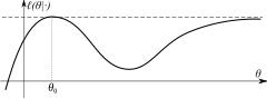
식별 조건에 따라 로그 우도가 고유한 글로벌 최대값을 갖는 것이 결정됩니다.콤팩트성은 우도가 다른 지점에서 임의로 가까운 최대값에 접근할 수 없음을 의미합니다(예: 오른쪽 그림).
콤팩트함은 충분한 조건일 뿐 필요한 조건은 아닙니다.콤팩트함은 다음과 같은 다른 조건으로 대체할 수 있습니다.
- 연속성: 함수 ln f(x µ)는 x의 거의 모든 값에 대해 θ에서 연속적입니다.
- 우위: 분포 f(x0 µ)와 관련하여 다음과 같이 적분 가능한 D(x)가 존재한다.


![{\displaystyle \operatorname {\mathbb {P} } {\Bigl [}\;\ln f(x\mid \theta )\;\in \;C^{0}(\Theta )\;{\Bigr ]}=1.}](https://wikimedia.org/api/rest_v1/media/math/render/svg/d3d9110b4a94639d23daa24b3cac7449a67ace0e)


우세 조건은 i.i.d. 관찰의 경우에 사용할 수 있다.non-i.d.의 경우, ( x) style ( \ style \ hat \ \ , , , ( \\ x )이 확률적으로 등가적이라는 것을 보여줌으로써 확률의 균일한 수렴을 확인할 수 있다.ML {\{\{\이(가) almost로0 거의 확실하게 수렴됨을 입증하려면 보다 강력한 균일한 수렴 조건을 적용해야 합니다.


또한 (위의 가정대로) 데이터가 f ; 0) { f _에 의해 생성된 경우에는 최대우도 추정기가 정규 분포로 수렴됨을 나타낼 수 있습니다.구체적으로는[18]

여기서 I는 피셔 정보 매트릭스입니다.
기능적 등변수
최대우도 추정기는 관측 데이터에 가능한 가장 큰 확률(또는 연속형인 경우 확률 밀도)을 제공하는 모수 값을 선택합니다.매개변수가 여러 성분으로 구성된 경우, 개별 최대우도 추정기를 전체 매개변수의 MLE에 해당하는 성분으로 정의한다.와 일관되게 이^({의 MLE이고 g가 \theta 의 변환인 경우 displaystyle\ta })의 MLE이 .


MLE는 데이터의 특정 변환에 대해서도 등변합니다.y () { y 여기서 g는 1 대 1이고 추정할 파라미터에 의존하지 않는 경우 함수는 다음을 만족합니다.

 1 대 1이고 추정할 파라미터에 의존하지 않는 경우
따라서 X X와 Y Y의 우도 함수는 모델 파라미터에 의존하지 않는 요인만 다를 뿐입니다.

 우도 함수는 모델 파라미터에 의존하지 않는 요인만 다를 뿐입니다.
 예를 들어, 로그 정규 분포의 MLE 모수는 데이터의 대수에 적합된 정규 분포의 모수와 동일합니다.
효율성.
위와 같이 데이터가 f ; {\~f(\0}~,})에 의해 생성되었을 경우, 최대우도 추정치가 정규 분포로 수렴됨을 알 수 있다.이 값은 µn 일관성이 있고 점근적으로 효율적이며, 이는 크라메르-라오 경계에 도달함을 의미한다.구체적으로는[18]
 의해 생성되었을 경우, 최대우도 추정치가 정규

![{\displaystyle {\mathcal {I}}_{jk}=\operatorname {\mathbb {E} } \,{\biggl [}\;-{\frac {\partial ^{2}\ln f_{\theta _{0}}(X_{t})}{\partial \theta _{j}\,\partial \theta _{k}}}\;{\biggr ]}~.}](https://wikimedia.org/api/rest_v1/media/math/render/svg/77f78bb077bde62448dcccfe59a51dcbb872c0bf)
특히, 최대우도 추정기의 치우침이 순서까지 0과 같다는 것을 의미합니다.1/160n.
바이어스 보정 후 2차 효율
그러나 이 추정기의 분포 확대에 있어서 고차항을 고려했을 때 has는mle 순서편향이 있음을 알 수 있다.1µn. 이 편향은 (성분별로)[20]와 같습니다.
![{\displaystyle b_{h}\;\equiv \;\operatorname {\mathbb {E} } {\biggl [}\;\left({\widehat {\theta }}_{\mathrm {mle} }-\theta _{0}\right)_{h}\;{\biggr ]}\;=\;{\frac {1}{\,n\,}}\,\sum _{i,j,k=1}^{m}\;{\mathcal {I}}^{hi}\;{\mathcal {I}}^{jk}\left({\frac {1}{\,2\,}}\,K_{ijk}\;+\;J_{j,ik}\right)}](https://wikimedia.org/api/rest_v1/media/math/render/svg/8340c5d355664078d79aeb28617e374438e8c60d)
서 I j {\위첨자 포함)는 역 피셔 정보 I - 의 (j,k)번째 컴포넌트를 나타냅니다.


![{\displaystyle {\frac {1}{\,2\,}}\,K_{ijk}\;+\;J_{j,ik}\;=\;\operatorname {\mathbb {E} } \,{\biggl [}\;{\frac {1}{2}}{\frac {\partial ^{3}\ln f_{\theta _{0}}(X_{t})}{\partial \theta _{i}\;\partial \theta _{j}\;\partial \theta _{k}}}+{\frac {\;\partial \ln f_{\theta _{0}}(X_{t})\;}{\partial \theta _{j}}}\,{\frac {\;\partial ^{2}\ln f_{\theta _{0}}(X_{t})\;}{\partial \theta _{i}\,\partial \theta _{k}}}\;{\biggr ]}~.}](https://wikimedia.org/api/rest_v1/media/math/render/svg/60eeb1b9aa84cb9d4ae9f0eb635f8d6a41a485fd)
이러한 공식을 사용하여 최대우도 추정기의 2차 편향을 추정할 수 있으며, 이를 빼서 편향을 보정할 수 있습니다.

이 추정치는 1/n 차수의 항까지 치우치지 않으며 치우침 보정 최대우도 추정기라고 합니다.
이 바이어스 보정 추정기는 2차 효율적이며(적어도 곡선 지수족 내), 즉 2차 바이어스 보정 추정기 중 1/n2 차수까지 최소 평균 제곱 오차를 가진다. 즉, 3차 바이어스 보정 항을 도출하는 등 이 과정을 계속할 수 있다.그러나 최대우도 추정기는 3차적으로 [21]효율적이지 않습니다.
베이지안 추론과의 관계
최대우도 추정기는 모수에 균일한 사전분포가 주어진 가장 가능성이 높은 베이지안 추정기와 일치한다.실제로, 최대 사후 추정치는 Bayes의 정리에 의해 주어진 데이터의 θ 확률을 최대화하는 매개변수 θ이다.

서 P ( ) { ( )는 파라미터 and의 이전 분포이며, ( 1, 2, x ){ style \ { \입니다.분모는 θ에 의존하지 않기 때문에 베이지안 추정치는 f1, 2, ) P ( ) \ f},)을 로 하여 구한다.의 P ( ) ( \\operatorname \ { P ( )이 균일한 분포라고 가정하면, 베이지안 추정치는 우도 f ( , 2, f를 최대화하여 얻을 수 있습니다.따라서 베이지안 추정치는 균일한 사전 P ( )의 최대우도 추정기와 일치한다
 파라미터
파라미터 

베이즈 의사결정 이론에서의 최대우도 추정 적용
기계 학습의 많은 실제 애플리케이션에서 최대우도 추정이 매개변수 추정을 위한 모델로 사용된다.
베이지안 결정 이론은 총 예상 위험을 최소화하는 분류기를 설계하는 것이다. 특히, 다른 결정과 관련된 비용(손실 함수)이 같을 때, 분류기는 전체 [22]분포에 걸쳐 오류를 최소화하는 것이다.
따라서 베이즈 의사결정 규칙은 다음과 같이 명시된다.
- "P ( x) > ( x) \ ( w _ { 1 x p pide \ \ ; w _ w _ { 1 x ) \ 。 이외의 경우 \;를 합니다.


서 w1, w 는 다른 클래스의 예측입니다.에러를 최소한으로 억제하는 관점에서는, 다음과 같이 말할 수도 있습니다.
 다른 클래스의 예측입니다.에러를 최소한으로 억제하는 관점에서는, 다음과 같이 말할 수도 있습니다.
어디에

2 P (오류 ) ( 2 \ ;\ x)=\ x if


베이즈의 정리를 적용하여
- w x wi) ) { P } ( w _ i \ x )= { \ w )
또한 모든 오류에 대해 동일한 손실인 제로 또는 1 손실 함수를 추가로 가정하면 베이즈 의사결정 규칙을 다음과 같이 재구성할 수 있습니다.
![{\displaystyle h_{\text{Bayes}}={\underset {w}{\operatorname {arg\;max} }}\,{\bigl [}\,\operatorname {\mathbb {P} } (x\mid w)\,\operatorname {\mathbb {P} } (w)\,{\bigr ]}\;,}](https://wikimedia.org/api/rest_v1/media/math/render/svg/a8946d22343b827b9f92e1bdd602bb4f99c8f379)
서 h Bayes는 예측값이고 P (w ) \ \ ;\\ {( w ) \ ; } the the the 。
 예측값이고 P
쿨백-라이블러 발산 및 교차 엔트로피 최소화와의 관계
을 최대화하는 을 찾는 것은 Kullback-Leibler의 관점에서 최소 거리를 갖는 확률 분포( 를 정의하는 를 찾는 것과 점근적으로 동등합니다.e, 데이터가 생성된 실제 확률 분포(즉, P 0 {\P_{\ _[23]에 생성됨).이상적인 세계에서는 P와 Q는 동일하지만(P를 정의하는 은 뿐입니다), P를 정의하는 것은 「\displaystyle\theta」뿐입니다만, 그것이 아니고, 사용하는 모델이 잘못 지정되어 있는 경우에서도, MLE는 에 모델 Q의 가장 가까운 를 제공합니다e P 0 { P _ { \ _ { } [24] 。


| 증거. |
| 간단한 표기법을 위해 P=Q라고 가정해 보겠습니다.y~ † { y P_의 의 i.i.d 데이터 y ( 1,, , n \} = ( {2} , , y {n} )가 있다고 합니다. ( \ P _ { \ )를 나서, 다음과 같이 합니다. 서 h ( x ) logP ( ) ( ∣ ) = \ { ( \ \ { }}{ ( \ \ theta h 를 사용하면 큰 수의 평균이 어떻게 이동하는지 알 수 있습니다.첫 번째 몇 가지 전환은 로그의 법칙과 관련이 있으며, 일부 함수를 최대화하는^(\을 찾는 것도 해당 함수의 단조로운 변환(즉, 상수 더하기/곱하기)을 극대화하는 것입니다. |
 있다고
있다고 
![{\displaystyle {\begin{aligned}{\hat {\theta }}&={\underset {\theta }{\operatorname {arg\,max} }}\,L_{P_{\theta }}(\mathbf {y} )={\underset {\theta }{\operatorname {arg\,max} }}\,P_{\theta }(\mathbf {y} )={\underset {\theta }{\operatorname {arg\,max} }}\,P(\mathbf {y} \mid \theta )\\&={\underset {\theta }{\operatorname {arg\,max} }}\,\prod _{i=1}^{n}P(y_{i}\mid \theta )={\underset {\theta }{\operatorname {arg\,max} }}\,\sum _{i=1}^{n}\log P(y_{i}\mid \theta )\\&={\underset {\theta }{\operatorname {arg\,max} }}\,\left(\sum _{i=1}^{n}\log P(y_{i}\mid \theta )-\sum _{i=1}^{n}\log P(y_{i}\mid \theta _{0})\right)={\underset {\theta }{\operatorname {arg\,max} }}\,\sum _{i=1}^{n}\left(\log P(y_{i}\mid \theta )-\log P(y_{i}\mid \theta _{0})\right)\\&={\underset {\theta }{\operatorname {arg\,max} }}\,\sum _{i=1}^{n}\log {\frac {P(y_{i}\mid \theta )}{P(y_{i}\mid \theta _{0})}}={\underset {\theta }{\operatorname {arg\,min} }}\,\sum _{i=1}^{n}\log {\frac {P(y_{i}\mid \theta _{0})}{P(y_{i}\mid \theta )}}={\underset {\theta }{\operatorname {arg\,min} }}\,{\frac {1}{n}}\sum _{i=1}^{n}\log {\frac {P(y_{i}\mid \theta _{0})}{P(y_{i}\mid \theta )}}\\&={\underset {\theta }{\operatorname {arg\,min} }}\,{\frac {1}{n}}\sum _{i=1}^{n}h_{\theta }(y_{i})\quad {\underset {n\to \infty }{\longrightarrow }}\quad {\underset {\theta }{\operatorname {arg\,min} }}\,E[h_{\theta }(y)]\\&={\underset {\theta }{\operatorname {arg\,min} }}\,\int P_{\theta _{0}}(y)h_{\theta }(y)dy={\underset {\theta }{\operatorname {arg\,min} }}\,\int P_{\theta _{0}}(y)\log {\frac {P(y\mid \theta _{0})}{P(y\mid \theta )}}dy\\&={\underset {\theta }{\operatorname {arg\,min} }}\,D_{\text{KL}}(P_{\theta _{0}}\parallel P_{\theta })\end{aligned}}}](https://wikimedia.org/api/rest_v1/media/math/render/svg/9c2c8b560e4cc7f5d9d1584e7361c86fb7db2f2b)

교차 엔트로피는 섀넌의 엔트로피 + KL 발산일 뿐이고, P 0style _의 엔트로피가 일정하므로 MLE는 교차 [25]엔트로피를 점근적으로 최소화하고 있다.
예
이산 균등 분포
1 ~ n의 번호가 매겨진 티켓이 1개씩 상자에 담겨져 랜덤으로 선택되는 경우(균등분포 참조), 샘플사이즈는 1 입니다.n이 불분명한 경우 n의 최대우도 추정기 {은 추첨된 티켓의 숫자 m입니다(n < m의 경우 0, n µ m의 경우 1µn, n = m의 경우 최대우도입니다).n의 최대우도 추정치는 가능한 값 범위의 "중간"이 아닌 가능한 값 {m, m + 1, ...}의 하한 극단에서 발생하므로 편향이 줄어듭니다.)추첨된 티켓의 숫자 m의 예상값, 즉 n의 예상값은 (n + 1)/2 입니다.결과적으로 표본 크기가 1인 경우 n에 대한 최대우도 추정기는 체계적으로 n을 (n - 1)/2만큼 과소평가합니다.
 추첨된 티켓의 숫자 m입니다(n < m의 경우 0, n
 이산 분포, 유한 모수 공간
어떤 사람이 부당한 동전이 얼마나 편파적인지 판단하고 싶다고 가정해 보자.'머리'를 던질 확률을 p라고 합니다.그런 다음 p를 결정하는 것이 목표가 됩니다.
동전을 80회 던졌다고 가정합니다. 즉, 샘플은 x = H, x2 = T, ..., x80 = T와1 같을 수 있으며 헤드 수 "H"의 카운트가 관찰됩니다.
꼬리를 던질 확률은 1 - p입니다(여기서 p는 위에 θ).결과가 49개의 앞면과 31개의 뒷면이라고 가정하고, 동전은 세 개의 동전이 들어 있는 상자에서 가져왔다고 가정합니다. 하나는 앞면이 p = 1⁄3이고, 하나는 앞면이 p = 2⁄2이고 다른 하나는 앞면이 p = 2⁄3입니다.그 동전들은 라벨을 잃어버렸기 때문에 어떤 것이었는지는 알 수 없다.최대우도 추정을 사용하면 관측된 데이터를 고려할 때 가장 높은 우도를 가진 동전을 찾을 수 있습니다.표본 크기가 80, 성공 횟수가 49인 이항 분포의 확률 질량 함수를 사용하여 p 값이 다른 경우("성공 확률") 우도 함수(아래 정의됨)는 세 가지 값 중 하나를 취합니다.
![{\displaystyle {\begin{aligned}\operatorname {\mathbb {P} } {\bigl [}\;\mathrm {H} =49\mid p={\tfrac {1}{3}}\;{\bigr ]}&={\binom {80}{49}}({\tfrac {1}{3}})^{49}(1-{\tfrac {1}{3}})^{31}\approx 0.000,\\[6pt]\operatorname {\mathbb {P} } {\bigl [}\;\mathrm {H} =49\mid p={\tfrac {1}{2}}\;{\bigr ]}&={\binom {80}{49}}({\tfrac {1}{2}})^{49}(1-{\tfrac {1}{2}})^{31}\approx 0.012,\\[6pt]\operatorname {\mathbb {P} } {\bigl [}\;\mathrm {H} =49\mid p={\tfrac {2}{3}}\;{\bigr ]}&={\binom {80}{49}}({\tfrac {2}{3}})^{49}(1-{\tfrac {2}{3}})^{31}\approx 0.054~.\end{aligned}}}](https://wikimedia.org/api/rest_v1/media/math/render/svg/547b3a227b1ae110fb6930d9dd0e586273e639f1)
p = 2⁄3일 때 우도가 최대화되므로 p에 대한 최대우도 추정치입니다.
이산 분포, 연속 모수 공간
이제 하나의 동전만 존재했지만 p는 임의의 값 0 p p 1 1이 될 수 있다고 가정합니다. 최대화 가능 함수는 다음과 같습니다.

최대화는 가능한 모든 값 0 p p 11에 대한 것입니다.

이 함수를 최대화하는 한 가지 방법은 p에 대해 차이를 두고 0으로 설정하는 것입니다.
![{\displaystyle {\begin{aligned}0&={\frac {\partial }{\partial p}}\left({\binom {80}{49}}p^{49}(1-p)^{31}\right)~,\\[8pt]0&=49p^{48}(1-p)^{31}-31p^{49}(1-p)^{30}\\[8pt]&=p^{48}(1-p)^{30}\left[49(1-p)-31p\right]\\[8pt]&=p^{48}(1-p)^{30}\left[49-80p\right]~.\end{aligned}}}](https://wikimedia.org/api/rest_v1/media/math/render/svg/11a8c9ed4cdd9536c6c56842e729a72bb71cdc3f)
This is a product of three terms. The first term is 0 when p = 0. The second is 0 when p = 1. The third is zero when p = 49⁄80. The solution that maximizes the likelihood is clearly p = 49⁄80 (since p = 0 and p = 1 result in a likelihood of 0). Thus the maximum likelihood estimator for p is 49⁄80.
This result is easily generalized by substituting a letter such as s in the place of 49 to represent the observed number of 'successes' of our Bernoulli trials, and a letter such as n in the place of 80 to represent the number of Bernoulli trials. Exactly the same calculation yields s⁄n which is the maximum likelihood estimator for any sequence of n Bernoulli trials resulting in s 'successes'.
Continuous distribution, continuous parameter space
For the normal distribution which has probability density function


the corresponding probability density function for a sample of n independent identically distributed normal random variables (the likelihood) is

This family of distributions has two parameters: θ = (μ, σ); so we maximize the likelihood, , over both parameters simultaneously, or if possible, individually.

Since the logarithm function itself is a continuous strictly increasing function over the range of the likelihood, the values which maximize the likelihood will also maximize its logarithm (the log-likelihood itself is not necessarily strictly increasing). The log-likelihood can be written as follows:

(Note: the log-likelihood is closely related to information entropy and Fisher information.)
We now compute the derivatives of this log-likelihood as follows.

where is the sample mean. This is solved by


This is indeed the maximum of the function, since it is the only turning point in μ and the second derivative is strictly less than zero. Its expected value is equal to the parameter μ of the given distribution,
![{\displaystyle \operatorname {\mathbb {E} } {\bigl [}\;{\widehat {\mu }}\;{\bigr ]}=\mu ,\,}](https://wikimedia.org/api/rest_v1/media/math/render/svg/29f9c10198da22e4e62bfaf33c49fcb08fcf9640)
which means that the maximum likelihood estimator is unbiased.

Similarly we differentiate the log-likelihood with respect to σ and equate to zero:

which is solved by

Inserting the estimate we obtain


To calculate its expected value, it is convenient to rewrite the expression in terms of zero-mean random variables (statistical error) . Expressing the estimate in these variables yields


Simplifying the expression above, utilizing the facts that and , allows us to obtain
![{\displaystyle \operatorname {\mathbb {E} } {\bigl [}\;\delta _{i}\;{\bigr ]}=0}](https://wikimedia.org/api/rest_v1/media/math/render/svg/d636e94e397dabd9c9247e3301e4cd6c26f3730a)
![{\displaystyle \operatorname {E} {\bigl [}\;\delta _{i}^{2}\;{\bigr ]}=\sigma ^{2}}](https://wikimedia.org/api/rest_v1/media/math/render/svg/f659be5d63a212a73928224e9b2f71e369bc2f44)
![{\displaystyle \operatorname {\mathbb {E} } {\bigl [}\;{\widehat {\sigma }}^{2}\;{\bigr ]}={\frac {\,n-1\,}{n}}\sigma ^{2}.}](https://wikimedia.org/api/rest_v1/media/math/render/svg/c2b9b5471de022ca37fa914e6f48fa38f489206c)
This means that the estimator is biased for . It can also be shown that is biased for , but that both and are consistent.


Formally we say that the maximum likelihood estimator for is


In this case the MLEs could be obtained individually. In general this may not be the case, and the MLEs would have to be obtained simultaneously.
The normal log-likelihood at its maximum takes a particularly simple form:

This maximum log-likelihood can be shown to be the same for more general least squares, even for non-linear least squares. This is often used in determining likelihood-based approximate confidence intervals and confidence regions, which are generally more accurate than those using the asymptotic normality discussed above.
Non-independent variables
It may be the case that variables are correlated, that is, not independent. Two random variables and are independent only if their joint probability density function is the product of the individual probability density functions, i.e.


Suppose one constructs an order-n Gaussian vector out of random variables , where each variable has means given by . Furthermore, let the covariance matrix be denoted by . The joint probability density function of these n random variables then follows a multivariate normal distribution given by:


![{\displaystyle f(y_{1},\ldots ,y_{n})={\frac {1}{(2\pi )^{n/2}{\sqrt {\det({\mathit {\Sigma }})}}}}\exp \left(-{\frac {1}{2}}\left[y_{1}-\mu _{1},\ldots ,y_{n}-\mu _{n}\right]{\mathit {\Sigma }}^{-1}\left[y_{1}-\mu _{1},\ldots ,y_{n}-\mu _{n}\right]^{\mathrm {T} }\right)}](https://wikimedia.org/api/rest_v1/media/math/render/svg/677eb0cae686c90d7da8e8f040a85d68f575d513)
In the bivariate case, the joint probability density function is given by:
![{\displaystyle f(y_{1},y_{2})={\frac {1}{2\pi \sigma _{1}\sigma _{2}{\sqrt {1-\rho ^{2}}}}}\exp \left[-{\frac {1}{2(1-\rho ^{2})}}\left({\frac {(y_{1}-\mu _{1})^{2}}{\sigma _{1}^{2}}}-{\frac {2\rho (y_{1}-\mu _{1})(y_{2}-\mu _{2})}{\sigma _{1}\sigma _{2}}}+{\frac {(y_{2}-\mu _{2})^{2}}{\sigma _{2}^{2}}}\right)\right]}](https://wikimedia.org/api/rest_v1/media/math/render/svg/9251f77c3cfe253bdf5ef19bf6bb3a8b09266293)
In this and other cases where a joint density function exists, the likelihood function is defined as above, in the section "principles," using this density.
Example
are counts in cells / boxes 1 up to m; each box has a different probability (think of the boxes being bigger or smaller) and we fix the number of balls that fall to be :. The probability of each box is , with a constraint: . This is a case in which the s are not independent, the joint probability of a vector is called the multinomial and has the form:


Each box taken separately against all the other boxes is a binomial and this is an extension thereof.
The log-likelihood of this is:

The constraint has to be taken into account and use the Lagrange multipliers:

By posing all the derivatives to be 0, the most natural estimate is derived

Maximizing log likelihood, with and without constraints, can be an unsolvable problem in closed form, then we have to use iterative procedures.
Iterative procedures
Except for special cases, the likelihood equations

cannot be solved explicitly for an estimator . Instead, they need to be solved iteratively: starting from an initial guess of (say ), one seeks to obtain a convergent sequence . Many methods for this kind of optimization problem are available,[26][27] but the most commonly used ones are algorithms based on an updating formula of the form


where the vector indicates the descent direction of the rth "step," and the scalar captures the "step length,"[28][29] also known as the learning rate.[30] In general the likelihood function is non-convex with multiple local maxima. Derivative based deterministic search methods can usually identify only a local maximum of the likelihood function. Locating a global maximum of a non-convex function is a NP-complete problem and hence cannot be solved within a reasonable time. Biologically inspired and other heuristic based optimization techniques can be used to explore multiple local maxima and identify an acceptable maximum in practice.[31]


Gradient descent method
(Note: here it is a maximization problem, so the sign before gradient is flipped)
- that is small enough for convergence and


Gradient descent method requires to calculate the gradient at the rth iteration, but no need to calculate the inverse of second-order derivative, i.e., the Hessian matrix. Therefore, it is computationally faster than Newton-Raphson method.
Newton–Raphson method
- and


where is the score and is the inverse of the Hessian matrix of the log-likelihood function, both evaluated the rth iteration.[32][33] But because the calculation of the Hessian matrix is computationally costly, numerous alternatives have been proposed. The popular Berndt–Hall–Hall–Hausman algorithm approximates the Hessian with the outer product of the expected gradient, such that


![{\displaystyle \mathbf {d} _{r}\left({\widehat {\theta }}\right)=-\left[{\frac {1}{n}}\sum _{t=1}^{n}{\frac {\partial \ell (\theta ;\mathbf {y} )}{\partial \theta }}\left({\frac {\partial \ell (\theta ;\mathbf {y} )}{\partial \theta }}\right)^{\mathsf {T}}\right]^{-1}\mathbf {s} _{r}\left({\widehat {\theta }}\right)}](https://wikimedia.org/api/rest_v1/media/math/render/svg/54504adfda94cd3accf328fc3a245468140acd35)
Quasi-Newton methods
Other quasi-Newton methods use more elaborate secant updates to give approximation of Hessian matrix.
Davidon–Fletcher–Powell formula
DFP formula finds a solution that is symmetric, positive-definite and closest to the current approximate value of second-order derivative:

where


Broyden–Fletcher–Goldfarb–Shanno algorithm
BFGS also gives a solution that is symmetric and positive-definite:

where
BFGS method is not guaranteed to converge unless the function has a quadratic Taylor expansion near an optimum. However, BFGS can have acceptable performance even for non-smooth optimization instances
Fisher's scoring
Another popular method is to replace the Hessian with the Fisher information matrix, , giving us the Fisher scoring algorithm. This procedure is standard in the estimation of many methods, such as generalized linear models.
![{\displaystyle {\mathcal {I}}(\theta )=\operatorname {\mathbb {E} } \left[\mathbf {H} _{r}\left({\widehat {\theta }}\right)\right]}](https://wikimedia.org/api/rest_v1/media/math/render/svg/79b549416c9863d8a2f90c6c50bbec905823ab21)
Although popular, quasi-Newton methods may converge to a stationary point that is not necessarily a local or global maximum,[34] but rather a local minimum or a saddle point. Therefore, it is important to assess the validity of the obtained solution to the likelihood equations, by verifying that the Hessian, evaluated at the solution, is both negative definite and well-conditioned.[35]
History

Early users of maximum likelihood were Carl Friedrich Gauss, Pierre-Simon Laplace, Thorvald N. Thiele, and Francis Ysidro Edgeworth.[36][37] However, its widespread use rose between 1912 and 1922 when Ronald Fisher recommended, widely popularized, and carefully analyzed maximum-likelihood estimation (with fruitless attempts at proofs).[38]
Maximum-likelihood estimation finally transcended heuristic justification in a proof published by Samuel S. Wilks in 1938, now called Wilks' theorem.[39] The theorem shows that the error in the logarithm of likelihood values for estimates from multiple independent observations is asymptotically χ 2-distributed, which enables convenient determination of a confidence region around any estimate of the parameters. The only difficult part of Wilks’ proof depends on the expected value of the Fisher information matrix, which is provided by a theorem proven by Fisher.[40] Wilks continued to improve on the generality of the theorem throughout his life, with his most general proof published in 1962.[41]
Reviews of the development of maximum likelihood estimation have been provided by a number of authors.[42][43][44][45][46][47][48][49]
See also
Related concepts
- Akaike information criterion: a criterion to compare statistical models, based on MLE
- Extremum estimator: a more general class of estimators to which MLE belongs
- Fisher information: information matrix, its relationship to covariance matrix of ML estimates
- Mean squared error: a measure of how 'good' an estimator of a distributional parameter is (be it the maximum likelihood estimator or some other estimator)
- RANSAC: a method to estimate parameters of a mathematical model given data that contains outliers
- Rao–Blackwell theorem: yields a process for finding the best possible unbiased estimator (in the sense of having minimal mean squared error); the MLE is often a good starting place for the process
- Wilks’ theorem: provides a means of estimating the size and shape of the region of roughly equally-probable estimates for the population's parameter values, using the information from a single sample, using a chi-squared distribution
Other estimation methods
- Generalized method of moments: methods related to the likelihood equation in maximum likelihood estimation
- M-estimator: an approach used in robust statistics
- Maximum a posteriori (MAP) estimator: for a contrast in the way to calculate estimators when prior knowledge is postulated
- Maximum spacing estimation: a related method that is more robust in many situations
- Maximum entropy estimation
- Method of moments (statistics): another popular method for finding parameters of distributions
- Method of support, a variation of the maximum likelihood technique
- Minimum distance estimation
- Partial likelihood methods for panel data
- Quasi-maximum likelihood estimator: an MLE estimator that is misspecified, but still consistent
- Restricted maximum likelihood: a variation using a likelihood function calculated from a transformed set of data
References
- ^ Rossi, Richard J. (2018). Mathematical Statistics : An Introduction to Likelihood Based Inference. New York: John Wiley & Sons. p. 227. ISBN 978-1-118-77104-4.
- ^ Hendry, David F.; Nielsen, Bent (2007). Econometric Modeling: A Likelihood Approach. Princeton: Princeton University Press. ISBN 978-0-691-13128-3.
- ^ Chambers, Raymond L.; Steel, David G.; Wang, Suojin; Welsh, Alan (2012). Maximum Likelihood Estimation for Sample Surveys. Boca Raton: CRC Press. ISBN 978-1-58488-632-7.
- ^ Ward, Michael Don; Ahlquist, John S. (2018). Maximum Likelihood for Social Science : Strategies for Analysis. New York: Cambridge University Press. ISBN 978-1-107-18582-1.
- ^ Press, W.H.; Flannery, B.P.; Teukolsky, S.A.; Vetterling, W.T. (1992). "Least Squares as a Maximum Likelihood Estimator". Numerical Recipes in FORTRAN: The Art of Scientific Computing (2nd ed.). Cambridge: Cambridge University Press. pp. 651–655. ISBN 0-521-43064-X.
- ^ Myung, I.J. (2003). "Tutorial on maximum likelihood Estimation". Journal of Mathematical Psychology. 47 (1): 90–100. doi:10.1016/S0022-2496(02)00028-7.
- ^ Gourieroux, Christian; Monfort, Alain (1995). Statistics and Econometrics Models. Cambridge University Press. p. 161. ISBN 0-521-40551-3.
- ^ Kane, Edward J. (1968). Economic Statistics and Econometrics. New York, NY: Harper & Row. p. 179.
- ^ Small, Christoper G.; Wang, Jinfang (2003). "Working with roots". Numerical Methods for Nonlinear Estimating Equations. Oxford University Press. pp. 74–124. ISBN 0-19-850688-0.
- ^ Kass, Robert E.; Vos, Paul W. (1997). Geometrical Foundations of Asymptotic Inference. New York, NY: John Wiley & Sons. p. 14. ISBN 0-471-82668-5.
- ^ Papadopoulos, Alecos (25 September 2013). "Why we always put log() before the joint pdf when we use MLE (Maximum likelihood Estimation)?". Stack Exchange.
- ^ a b Silvey, S. D. (1975). Statistical Inference. London, UK: Chapman and Hall. p. 79. ISBN 0-412-13820-4.
- ^ Olive, David (2004). "Does the MLE maximize the likelihood?" (PDF).
{{cite journal}}: Cite journal requiresjournal=(help) - ^ Schwallie, Daniel P. (1985). "Positive definite maximum likelihood covariance estimators". Economics Letters. 17 (1–2): 115–117. doi:10.1016/0165-1765(85)90139-9.
- ^ Magnus, Jan R. (2017). Introduction to the Theory of Econometrics. Amsterdam: VU University Press. pp. 64–65. ISBN 978-90-8659-766-6.
- ^ Pfanzagl (1994, p. 206)
- ^ By Theorem 2.5 in Newey, Whitney K.; McFadden, Daniel (1994). "Chapter 36: Large sample estimation and hypothesis testing". In Engle, Robert; McFadden, Dan (eds.). Handbook of Econometrics, Vol.4. Elsevier Science. pp. 2111–2245. ISBN 978-0-444-88766-5.
- ^ a b By Theorem 3.3 in Newey, Whitney K.; McFadden, Daniel (1994). "Chapter 36: Large sample estimation and hypothesis testing". In Engle, Robert; McFadden, Dan (eds.). Handbook of Econometrics, Vol.4. Elsevier Science. pp. 2111–2245. ISBN 978-0-444-88766-5.
- ^ Zacks, Shelemyahu (1971). The Theory of Statistical Inference. New York: John Wiley & Sons. p. 223. ISBN 0-471-98103-6.
- ^ See formula 20 in Cox, David R.; Snell, E. Joyce (1968). "A general definition of residuals". Journal of the Royal Statistical Society, Series B. 30 (2): 248–275. JSTOR 2984505.
- ^ Kano, Yutaka (1996). "Third-order efficiency implies fourth-order efficiency". Journal of the Japan Statistical Society. 26: 101–117. doi:10.14490/jjss1995.26.101.
- ^ Christensen, Henrikt I. "Pattern Recognition" (PDF) (lecture). Bayesian Decision Theory - CS 7616. Georgia Tech.
- ^ cmplx96 (https://stats.stackexchange.com/users/177679/cmplx96), Kullback–Leibler divergence, URL (version: 2017-11-18): https://stats.stackexchange.com/q/314472 (at the youtube video, look at minutes 13 to 25)
- ^ Introduction to Statistical Inference Stanford (Lecture 16 — MLE under model misspecification)
- ^ Sycorax says Reinstate Monica (https://stats.stackexchange.com/users/22311/sycorax-says-reinstate-monica), the relationship between maximizing the likelihood and minimizing the cross-entropy, URL (version: 2019-11-06): https://stats.stackexchange.com/q/364237
- ^ Fletcher, R. (1987). Practical Methods of Optimization (Second ed.). New York, NY: John Wiley & Sons. ISBN 0-471-91547-5.
- ^ Nocedal, Jorge; Wright, Stephen J. (2006). Numerical Optimization (Second ed.). New York, NY: Springer. ISBN 0-387-30303-0.
- ^ Daganzo, Carlos (1979). Multinomial Probit : The Theory and its Application to Demand Forecasting. New York: Academic Press. pp. 61–78. ISBN 0-12-201150-3.
- ^ Gould, William; Pitblado, Jeffrey; Poi, Brian (2010). Maximum Likelihood Estimation with Stata (Fourth ed.). College Station: Stata Press. pp. 13–20. ISBN 978-1-59718-078-8.
- ^ Murphy, Kevin P. (2012). Machine Learning: A Probabilistic Perspective. Cambridge: MIT Press. p. 247. ISBN 978-0-262-01802-9.
- ^ Noel, M.M.; Joshi, P.P.; Jannett, T.C. (April 2006). "Improved Maximum Likelihood Estimation of Target Position in Wireless Sensor Networks using Particle Swarm Optimization". Third International Conference on Information Technology: New Generations (ITNG'06): 274–279. doi:10.1109/ITNG.2006.72. ISBN 0-7695-2497-4. S2CID 17322072.
- ^ Amemiya, Takeshi (1985). Advanced Econometrics. Cambridge: Harvard University Press. pp. 137–138. ISBN 0-674-00560-0.
- ^ Sargan, Denis (1988). "Methods of Numerical Optimization". Lecture Notes on Advanced Econometric Theory. Oxford: Basil Blackwell. pp. 161–169. ISBN 0-631-14956-2.
- ^ See theorem 10.1 in Avriel, Mordecai (1976). Nonlinear Programming: Analysis and Methods. Englewood Cliffs, NJ: Prentice-Hall. pp. 293–294. ISBN 9780486432274.
- ^ Gill, Philip E.; Murray, Walter; Wright, Margaret H. (1981). Practical Optimization. London, UK: Academic Press. pp. 312–313. ISBN 0-12-283950-1.
- ^ Edgeworth, Francis Y. (Sep 1908). "On the probable errors of frequency-constants". Journal of the Royal Statistical Society. 71 (3): 499–512. doi:10.2307/2339293. JSTOR 2339293.
- ^ Edgeworth, Francis Y. (Dec 1908). "On the probable errors of frequency-constants". Journal of the Royal Statistical Society. 71 (4): 651–678. doi:10.2307/2339378. JSTOR 2339378.
- ^ Pfanzagl, Johann; Hamböker, R. (1994). Parametric Statistical Theory. Walter de Gruyter. pp. 207–208. ISBN 978-3-11-013863-4.
- ^ Wilks, S.S. (1938). "The large-sample distribution of the likelihood ratio for testing composite hypotheses". Annals of Mathematical Statistics. 9: 60–62. doi:10.1214/aoms/1177732360.
- ^ Owen, Art B. (2001). Empirical Likelihood. London, UK; Boca Raton, FL: Chapman & Hall; CRC Press. ISBN 978-1584880714.
- ^ Wilks, Samuel S. (1962). Mathematical Statistics. New York, NY: John Wiley & Sons. ISBN 978-0471946502.
- ^ Savage, Leonard J. (1976). "On rereading R.A. Fisher". The Annals of Statistics. 4 (3): 441–500. doi:10.1214/aos/1176343456. JSTOR 2958221.
- ^ Pratt, John W. (1976). "F. Y. Edgeworth and R. A. Fisher on the efficiency of maximum likelihood estimation". The Annals of Statistics. 4 (3): 501–514. doi:10.1214/aos/1176343457. JSTOR 2958222.
- ^ Stigler, Stephen M. (1978). "Francis Ysidro Edgeworth, statistician". Journal of the Royal Statistical Society, Series A. 141 (3): 287–322. doi:10.2307/2344804. JSTOR 2344804.
- ^ Stigler, Stephen M. (1986). The history of statistics: the measurement of uncertainty before 1900. Harvard University Press. ISBN 978-0-674-40340-6.
- ^ Stigler, Stephen M. (1999). Statistics on the table: the history of statistical concepts and methods. Harvard University Press. ISBN 978-0-674-83601-3.
- ^ Hald, Anders (1998). A history of mathematical statistics from 1750 to 1930. New York, NY: Wiley. ISBN 978-0-471-17912-2.
- ^ Hald, Anders (1999). "On the history of maximum likelihood in relation to inverse probability and least squares". Statistical Science. 14 (2): 214–222. doi:10.1214/ss/1009212248. JSTOR 2676741.
- ^ Aldrich, John (1997). "R.A. Fisher and the making of maximum likelihood 1912–1922". Statistical Science. 12 (3): 162–176. doi:10.1214/ss/1030037906. MR 1617519.
Further reading
- Cramer, J.S. (1986). Econometric Applications of Maximum Likelihood Methods. New York, NY: Cambridge University Press. ISBN 0-521-25317-9.
- Eliason, Scott R. (1993). Maximum Likelihood Estimation : Logic and Practice. Newbury Park: Sage. ISBN 0-8039-4107-2.
- King, Gary (1989). Unifying Political Methodology : the Likehood Theory of Statistical Inference. Cambridge University Press. ISBN 0-521-36697-6.
- Le Cam, Lucien (1990). "Maximum likelihood : An Introduction". ISI Review. 58 (2): 153–171. doi:10.2307/1403464. JSTOR 1403464.
- Magnus, Jan R. (2017). "Maximum Likelihood". Introduction to the Theory of Econometrics. Amsterdam, NL: VU University Press. pp. 53–68. ISBN 978-90-8659-766-6.
- Millar, Russell B. (2011). Maximum Likelihood Estimation and Inference. Hoboken, NJ: Wiley. ISBN 978-0-470-09482-2.
- Pickles, Andrew (1986). An Introduction to Likelihood Analysis. Norwich: W. H. Hutchins & Sons. ISBN 0-86094-190-6.
- Severini, Thomas A. (2000). Likelihood Methods in Statistics. New York, NY: Oxford University Press. ISBN 0-19-850650-3.
- Ward, Michael D.; Ahlquist, John S. (2018). Maximum Likelihood for Social Science : Strategies for Analysis. Cambridge University Press. ISBN 978-1-316-63682-4.
External links
- Lesser, Lawrence M. (2007). "'MLE' song lyrics". Mathematical Sciences / College of Science. math.utep.edu. El Paso, TX: University of Texas. Retrieved 2021-03-06.
{{cite web}}: CS1 maint: url-status (link) - "Maximum-likelihood method", Encyclopedia of Mathematics, EMS Press, 2001 [1994]
- Purcell, S. "Maximum Likelihood Estimation".
- Sargent, Thomas; Stachurski, John. "Maximum Likelihood Estimation". Quantitative Economics with Python.
- Toomet, Ott; Henningsen, Arne (2019-05-19). "maxLik: A package for maximum likelihood estimation in R".